
- Definition of the Triaural acoustic resonator, taxonomy, cymatics, safety, and ethics
- Expanded research proposal and technical requirements for the research facility
- Analysis of financing as an open opportunity
INTRODUCTORY WORD
TRIAURAL began with a simple question that unexpectedly opened a much wider field of questions. What changes when the familiar two-pronged tuning fork is extended by a third prong and its geometry gains spatial symmetry? Sometimes a small change in shape is enough to turn a familiar object into a new research question.
This idea gradually became the subject of informal discussions with artificial intelligence (AI) language models at the intersection of mechanics, acoustics, geometry, materials, and wave-field structure. This document captures the stage at which the original idea is being transformed into a precisely defined research problem.
The preceding dialogues and question-based documents form the exploratory layer of the project. Their purpose was to map possible directions, connections, and boundaries of the topic without claiming experimental confirmation. Research programs N1-N3 build on this exploratory work in a different mode: hypotheses, methods, measurable quantities, and falsification criteria are formulated so that they can be tested independently. The exploratory material remains preserved as a record of how the questions emerged; research status subsequently follows from the methodological and experimental procedures defined in these programs.
This document was created outside the academic environment. It is not backed by institutions, university departments, or grants, and at the time of publication it has no systematic measurements on which to rely. For that reason, it places even greater emphasis on clearly defining the subject, using consistent terminology, distinguishing the evidential weight of claims, and formulating questions in a way that allows experimental testing.
The text therefore clearly separates documented knowledge, observations, hypotheses, and visions. Decisive claims are tied to measurable quantities, and hypotheses to conditions that allow rigorous evaluation.
N1 is the first methodological framework in a three-part research compendium. Its purpose is to establish a common foundation for further measurement, modeling, independent verification, and open discussion.
The following pages are a map of questions awaiting experimental answers.
- TRIAURAL -
CONTENTS
- 01 ABSTRACT AND STATUS OF THE DOCUMENT
- 02 ORIGIN OF THE TERM TRIAURAL
- 03 SYSTEM DEFINITION
- 04 COMPLEXITY LADDER L0 - L7
- 05 DEVICE CLASSIFICATION
- 06 GEOMETRIC DESCRIPTION
- 07 NORMATIVE TERMINOLOGY
- 08 DEFINITION OF ANGULAR PARAMETERS
- 09 PHYSICAL BASIS
- 10 CYMATICS AND THE ACOUSTIC HOLOGRAM - A FIELD THAT CAN BE SEEN AND HEARD
- 11 WATER AND LIQUID MEDIA
- 12 MULTI-SOURCE FIELD SYNTHESIS
- 13 NON-CONTACT EXCITATION AND SENSING
- 14 HANDLE AS A WAVEGUIDE
- 15 MATERIAL BASE
- 16 MATHEMATICAL RELATIONS
- 17 COMPUTATIONAL MODEL AND VALIDATION
- 18 SAFETY, DOSIMETRY, AND ETHICS
- 19 EQUIPMENT AND ESTIMATED COSTS
- 20 DESIGN OF THE RESEARCH FACILITY
- 21 TIMELINE
- 22 HYPOTHESES
- 23 FINANCING ANALYSIS AND OPEN OPPORTUNITY
- 24 SUMMARY AND OPEN CALL
- P APPENDICES AND SOURCES
ABSTRACT AND STATUS OF THE DOCUMENT
This chapter explains why the document was created, who it is intended for, and what can reasonably be expected from it. Anyone who continues reading should come away knowing exactly where measured evidence ends and where ideas that are still being considered begin.
1.1 Purpose of the document
The purpose of this document is to establish a firm definitional foundation for Triaural resonators - to state exactly what is being studied, what terminology is used to describe it, and which quantities are used to measure it.
This document is not a grant application, although it includes a budget analysis. Nor is it a presentation of completed results, because no systematic measurements yet exist. It is a foundation that anyone wishing to continue work on this topic can use - including researchers with no connection to the TRIAURAL team who want to examine our assumptions independently.
We therefore do not define the success of this document by whether it persuades. We define success by whether, after reading it, a person can state exactly which experiment would decide the matter - and what result would be required to show that we are wrong.
Three practical objectives follow from this:
- Standardize the terminology so that two independent teams use the same words for the same object.
- Separate claims according to the strength of their support and make that distinction visible throughout the text.
- Formulate the questions so that each can ultimately be answered by a measurable quantity.
1.2 Position within the twelve-document series
The document designated N1 is the tenth document in the publication series. The first nine documents record questions posed to AI models and their responses; they form the exploratory layer of the publication series and should be read as such. Documents ten through twelve (N1-N3) form the project's formal research line and represent the position of the TRIAURAL team.
The individual parts of the series are referred to as nodes. A node is a self-contained research unit with its own subject, budget, and document; this document describes Node N1.
In this document, the term project refers to the overarching TRIAURAL research framework. The individual nodes N1, N2, and N3 are referred to as research programs in organizational, implementation, and financial contexts. The TRIAURAL project therefore consists of research programs N1, N2, and N3.
N1 has a normative role within this group. This means that terminology and angular parameters are defined exclusively in this document and are not redefined in N2 or N3; where necessary, those documents refer back to N1. If a definition changes in the future, it changes in one place.
Document N2 addresses electromagnetic radiators, while N3 addresses the AURIS multiresonant chamber and questions related to the nervous system. Across the three documents, the degree of speculation increases as the amount of hard data decreases. N1 is therefore intentionally the most restrained and descriptive of the three.
1.3 Epistemic register and labeling
To make the evidential weight of each statement clear, every substantive claim carries one of four labels:
D) DOCUMENTED
Measured, recorded, or published. The method, instrument, and measurement conditions are stated, or a reference to the literature is provided. If this information is missing, the statement does not receive the [D] label, even if it happens to be true.
H) HYPOTHESIS
A falsifiable claim. It must include a testable criterion, a prediction, and - most importantly - a falsification criterion: a statement specifying what would have to be measured for the hypothesis to fail.
V) VISION
A statement that extends beyond current testability. It is presented openly and without apology. A vision is not a weaker hypothesis - it is a different category and is not treated as a hypothesis in this document.
O) OBSERVATION
A phenomenon that has been observed repeatedly, but without recorded conditions, without a control measurement, or without repetition in a comparable setup. It is not presented as a result and does not support a claim. It is included because it led to the formulation of a question.
The register and the item type are two different things. The registers [D], [O], [H], and [V] indicate the evidential weight of a statement. The item type indicates the kind of question being asked: a hypothesis identified as H-N1-xx asks whether something is true, while a question identified as Q-N1-xx asks how or why. Details are provided in Chapter N1/22.1.
In this edition, the [D] label applies exclusively to evidence from an external source - a peer-reviewed paper, patent, or standard. No original systematic measurements yet exist; once they do, they will be labeled separately so that the origin of the evidence can be distinguished without having to trace it through the document.
This distinction is a tool that allows bold ideas to be stated more clearly than would otherwise be possible. A vision labeled as a vision is not a result.
Hypotheses are numbered sequentially in the form H-N1-01, and once assigned, an identifier never changes. Each hypothesis is given a status (open, tested, confirmed, falsified, revised, unsupported) and the research phase to which it belongs. Cross-references between chapters use the form N1/07, or N1/07.3 for a subsection.
1.4 Preregistered and exploratory findings
Every finding belongs to one of two classes and must be labeled accordingly.
- A preregistered finding comes from a measurement specified in advance in the protocol. Its interpretation cannot be reformulated afterward to fit the outcome.
- An exploratory finding is anything else that emerges during measurement. It is fully legitimate and must be recorded; the only condition is that it is not presented as confirmation of a hypothesis.
Priority of hypotheses
The document contains more than sixty hypotheses, and without an ordering they would be difficult to use. Each therefore belongs to one of four groups.
- Decision hypothesis. Its result determines whether the program continues along a given branch. There are only a few, and they are listed below.
- Derived hypothesis. Tests a mechanism or parameter within a branch opened by a decision hypothesis.
- Conditional hypothesis. Becomes active only after a preceding condition has been met and is not tested before then.
- Exploratory hypothesis. A legitimate measurement without a preregistered criterion; its outcome is not presented as confirmation of a hypothesis under Chapter N1/01.4.
This document contains four decision hypotheses. They concern whether a three-pronged body has a pair of natural modes that a two-pronged body cannot have; whether its acoustic field can be distinguished from the field produced by an assembled set of three separate sources; the nature of the rotating component of that field; and whether the rotating state arises from the geometry of the body itself or must be imposed through the excitation method. They are introduced in Chapters N1/09 and N1/12 and are identified where they appear in the text.
Minimum preregistration requirements
For a decision hypothesis, five items are recorded before measurement: the primary measured quantity, confirmation criterion, falsification criterion, number of repetitions, and rules for excluding a measurement from the series. A falsification criterion is always required; a hypothesis that cannot be falsified is not a hypothesis.
If multiple quantities are evaluated simultaneously within a single hypothesis, this is specified in advance together with the method for handling multiple testing. Without this rule, almost any hypothesis could be confirmed simply by measuring enough quantities.
The preregistration record is versioned and attached to the published data. This minimum is not required for derived, conditional, or exploratory hypotheses.
The reason for this clause is historical and instructive. Sonoluminescence - the production of flashes of light in a liquid under acoustic excitation - was discovered in 1934 by Frenzel and Schultes when, while working on sonar, they noticed that photographic plates in the vessel were becoming fogged. They were not looking for light and had no hypothesis about it. A protocol with no room for anomalies would have dismissed such a finding as an artifact.
1.5 What the document does not claim
We consider it essential to state that negative delimitation is just as important as positive definition, which is why it appears at the beginning rather than at the end.
- The document does not claim that the Triaural resonator has therapeutic effects. It makes no health claims and is not a basis for a medical device.
- The document does not claim that a rotating field has been demonstrated. It explains why its existence is hypothesized and what measurements could confirm or rule it out.
- The document does not claim that the geometry of the resonator carries symbolic or nonphysical meaning. The angles 60°, 90°, 109.47°, and 120° are geometric parameters in this document, nothing more.
- The document does not use terms that lack a measurable definition. A list of such terms and the reasons for excluding them is provided in Appendix P4.
The document does not contain detailed measurement protocols specifying step-by-step procedures, instruments, and recording forms. Those protocols will be developed together with the measurements and published as part of the resulting outputs. The methodological requirements this document places on them are stated in the relevant chapters.
ORIGIN OF THE TERM TRIAURAL
Where did the idea come from, and why study a tuning fork with three prongs when two have worked reliably for more than three hundred years? This chapter also identifies what is most unusual about the entire project: this is not a new perspective on a familiar object, but an object that has not been systematically addressed in the scientific literature.
The term TRIAURAL originated on February 2, 2025, as a direct result of a dialogue between the project founder and the ChatGPT language model (OpenAI).
After the opening question, “What would happen if we added a third prong to a conventional two-pronged tuning fork...?”, the dialogue with ChatGPT produced the first toroidal hypothesis: the model estimated that a toroidal structure of acoustic energy could form between the prongs of a three-pronged tuning fork arranged in space at 120°. For the members of the TRIAURAL team, this statement served as an activation point - an internal intuition supported by a physically plausible hypothesis with potentially far-reaching implications.
After the initial question, a team member asked how the three-pronged tuning fork and the principle behind it might be named. The response was the term TRIAURAL, which was immediately adopted as a precise and resonant definition of the system.
Since that moment, an ongoing research dialogue has continued between the TRIAURAL team and several AI systems, including ChatGPT - OpenAI, Grok - xAI, Copilot - Microsoft, Claude - Anthropic, Gemini - Google DeepMind, and Kimi - Moonshot AI. This document is one product of that process.
This circumstance documents the origin of the terminology; it does not constitute evidence of the physical validity of the concept or its acceptance by the scientific community.
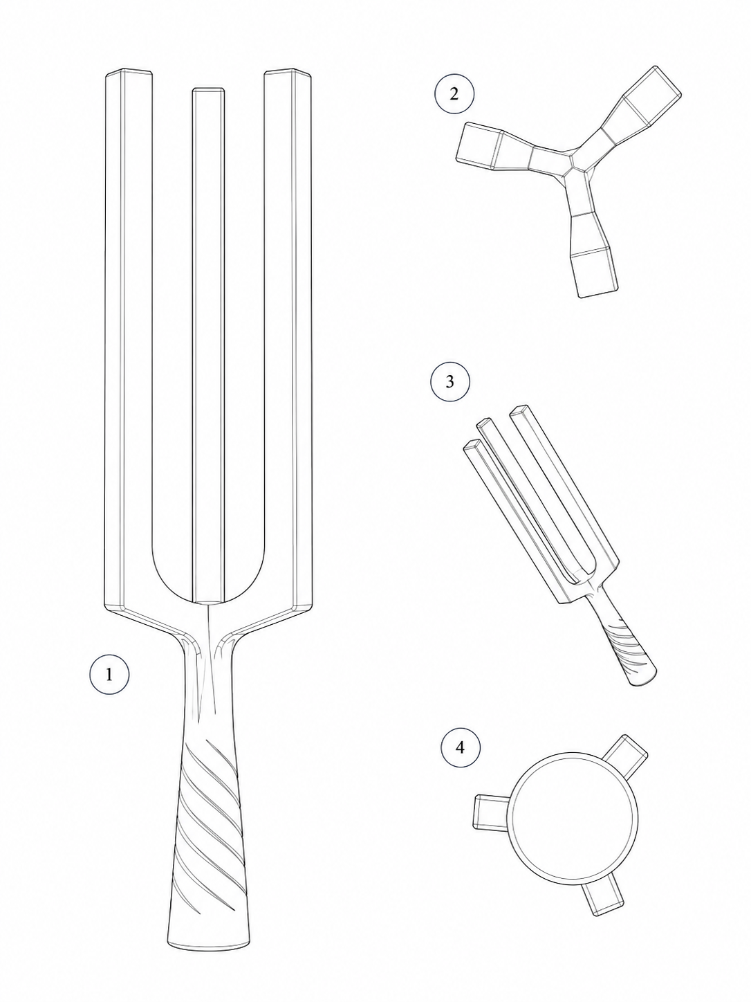
2.1 The two-pronged tuning fork and why it became the standard
The tuning fork in the form familiar to almost everyone originated in 1711. It was invented by the English trumpeter and lutenist John Shore, and its shape has remained practically unchanged ever since. [1] That is remarkable in itself - few instruments have survived three centuries without a fundamental change to their basic form.
The reason is not accidental and is worth stating clearly. The two prongs of a tuning fork vibrate symmetrically in opposition: as they open, both free ends move away from the central plane, and their transverse reactions at the common base act in opposite directions. These reactions largely cancel at the junction, so only a small transverse component of motion is transmitted into the handle. The handle therefore acts primarily in the longitudinal direction - which is why the sound becomes markedly louder when its base is pressed against a tabletop. [1]
The consequence is fundamental: the tuning fork loses very little energy into its support, so it rings for a long time and its pitch remains stable. Two-pronged geometry is therefore a highly efficient engineering form for one task - producing a pure, stable, long-lasting tone.
This is why it became the standard in acoustics and has been described in great detail. Its modes, ring-down, temperature dependence, and material effects belong to the basic inventory of the field.
2.2 What the third prong introduces
If two-pronged geometry is optimal for a single tone, the question naturally follows - why try three prongs?
The argument based on cancellation of transverse forces applies just as well to three prongs. If three prongs spaced 120° apart deflect symmetrically, their transverse reactions should largely cancel at the central node, and the resonator should lose similarly little energy into its mounting as a two-pronged tuning fork.
Three prongs, however, introduce a new element. Under ideal threefold C3 symmetry, the theory of rotationally periodic structures predicts, for the relevant nonsymmetric modal class, a pair of mutually independent mode shapes with the same natural frequency - a degenerate pair [18]. Put simply, the body can vibrate in this class in two different ways, neither of which is favored by the symmetry, so in the ideal case they have the same frequency. With an appropriate phase combination, they can form a rotating normal mode.
In a conventional two-pronged tuning fork, such a pair is not enforced by its C2 symmetry. In a real three-pronged resonator, moreover, the pair may not remain perfectly degenerate: manufacturing deviations, material asymmetries, or mounting conditions may split the pair in frequency. The existence of the pair and the magnitude of its splitting are therefore among the decisive quantities to be tested by modal analysis and subsequent measurement. A detailed derivation is given in Chapter N1/09.
It follows that a three-pronged resonator is not merely a tuning fork with one extra prong. It represents a different class of object that shares the basic structural principle of the two-pronged form, while its threefold symmetry allows a different modal structure and, with it, additional possible states of the resulting field.
2.3 What the literature says about related topics
To determine what may be new about Triaural resonators, it is first necessary to define precisely what is not new. The following areas are thoroughly covered in the scientific literature, and this project makes no claim to them:
- Vibration of rods, plates, and membranes, including two-pronged tuning forks. Classical theory extends back to nineteenth-century work and is well established.
- Axisymmetric resonators - bells, bowls, and cups - including their degenerate modes and the phenomenon of mode splitting.
- Acoustic vortices and the orbital angular momentum of sound. This is an established phenomenon with industrial applications; an overview of current generation methods is provided in Chapter N1/09.8.
- Phased transducer arrays and their control. These are standard techniques in both ultrasound and sound reinforcement.
- Tripole and crossed-dipole antennas in electromagnetics. These principles are well developed in antenna engineering and are addressed in greater detail in document N2.
Three-pronged tuning forks also appear commercially among instruments marketed for sound therapy under the designation trident. These designs, however, have their prongs in a single plane. Manufacturers justify them by greater mass and longer ring-down, and their descriptions specify frequency, material, and mass, but not angular parameters of a three-dimensional configuration.
A planar arrangement does not create the threefold radial C3 symmetry on which the degenerate pair examined in Chapter N1/09 is based. From the standpoint of this document, it therefore does not address the same subject, but rather a different construction with a different purpose.
Whether the three-dimensional threefold geometry of a resonator has already been systematically investigated in this form is not treated as predetermined in this document. It is the subject of a dedicated literature search. The search includes scientific databases, citation indexes, patent databases, historical literature, and available technical sources; the procedure, search queries, and limitations are described in Section 2.5.
The preliminary search showed that individual elements of the concept - multi-pronged tuning forks, rotational symmetry, degenerate modes, and acoustic vortices - all have precedents in the literature. Their combination as a research subject centered on a monolithic three-pronged resonator with three-dimensional C3 symmetry, however, did not appear in the sources identified to date as a distinct systematically studied topic. Such an absence does not in itself prove novelty; it does, however, represent a notable literature gap that the detailed search protocol is intended to confirm, refine, or refute.
The family of multi-pronged tuning forks also has a long patent history. U.S. Patent 2,601,801 from 1952 describes a three-tine tuning fork conceived as a set of nested two-pronged tuning forks sounding simultaneously. U.S. Patent 3,405,589, granted in 1968, claims a tuning fork with at least three tines, one of which is deliberately detuned to produce beats and tremolo; the patent also contemplates a four-tine version tuned to a harmonic triad of tones.
What matters is the purpose of these designs. They are intended to manipulate frequency - producing beats, tremolo, and chords - and therefore deliberately detune the tines. A Triaural resonator requires the closest possible match among its arms, because detuning splits the degenerate pair and suppresses the state under investigation. What is a design objective in those patents would constitute a manufacturing error in a Triaural resonator.
The existence of these solutions also shows why the search described in Section 2.5 cannot be limited to academic publications. Structural variations of tuning forks have historically appeared in patent literature, technical documents, and commercial implementations as well. Assessing possible precedent therefore requires comparison across several source types and, above all, comparison of their geometric and functional content rather than merely the device name or number of prongs.
2.4 What is missing from the literature
Despite the breadth of existing knowledge described above, we did not find a systematic treatment of the following area:
- Monolithic acoustic resonators with threefold or higher radial symmetry treated as a class of objects defined by angular parameters.
- Measurement of their near-field structure beyond angular radiation patterns, particularly the question of whether and under what conditions the field contains a rotating component.
- Normative terminology for their components and angles that would allow results to be compared across laboratories.
- The relationship between angular accuracy and the properties of the resulting field.
This is one of the most significant and, at the same time, most fragile claims in the entire document. It is significant because, if correct, it means that the project is not opening a new perspective on a familiar object, but addressing an object that may not yet have been systematically studied. It is fragile because a claim of nonexistence can never be proven completely. It therefore applies only within the scope of the freely accessible sources and patent databases listed in Section 2.5; the possibility always remains that relevant work exists and we did not find it.
Accordingly, the document nowhere states that such research does not exist. It states that we did not find it, and provides a record of how we searched.
2.5 Literature search protocol
For the claim in the preceding subsection to be verifiable and citable, the literature search must be documented in the same way as any other measurement. A negative result from a documented search is a legitimate result; an undocumented impression is not.
The search is therefore performed and recorded with the following information: databases used, exact query strings, date performed, number of records found, and the reason for excluding records unrelated to the subject.
- Bibliographic databases: Web of Science, Scopus, IEEE Xplore, the Journal of the Acoustical Society of America archive, Google Scholar.
- Patent databases: Espacenet, Patentscope, Google Patents. Patent literature is particularly important for this type of topic because structural solutions often appear in patent applications rather than in journal articles.
- Query groups: three-pronged and multi-pronged tuning forks, monolithic resonators with radial symmetry, degenerate modes under threefold symmetry, acoustic-vortex generation by passive geometry, and the near field of multi-pronged resonators.
Execution
The first search run was conducted on August 23, 2026. Fifteen exact English-language queries were run in Google Scholar and Semantic Scholar. Three queries concerning acoustic vortices and orbital angular momentum were run in arXiv, one structural query in Google Patents, and Espacenet was used to verify one patent record. On August 24, 2026, IEEE Xplore and the Journal of the Acoustical Society of America archive were added, followed by Scopus on August 25, 2026; the complete set of fifteen queries was run in all three of these sources.
Six AI systems were included in a parallel literature-search process with the same assignment and the same list of queries: Tasklet, Grok, Copilot, Gemini, Kimi, and Google Search answer mode. Kimi did not participate because its free mode was unavailable at the time of the search; its run is recorded as not performed, not as a zero-result search. Gemini did not have search access available and stated this instead of estimating results; its run is recorded in the same way.
This arrangement was chosen deliberately. Agreement among parallel runs increases confidence in the reproducibility of the findings, while disagreement highlights records requiring manual verification. There were more discrepancies than expected, so every bibliographically decisive record was verified against a primary source, meaning the publisher record or the full patent text. Only records that passed this verification were included.
The verification process is part of the protocol because it exposed errors that would otherwise have entered the document. One system paired the correct identifier with the wrong title. Another classified a patent as two-pronged even though its claim specifies three or more tines. For one group of papers, the systems disagreed on publication year, volume, and the name of the third author; it turned out that these were not three attempts to cite one paper, but three different papers by the same group, two of which could be verified.
The complete record of queries, counts, and database-specific notes is provided in Appendix N1/P5.
Included academic papers
- [2] Blodgett, E. D., McCann, L. I., Anderson, C.: Radiation patterns of novel one- and three-tine tuning forks. J. Acoust. Soc. Am. 110, 2730 (2001). DOI 10.1121/1.4777461. Abstract from the 142nd Meeting of the Acoustical Society of America.
- [3] Tamura, H., Takano, T., Tomikawa, Y.: Triaxial Quartz Gyrosensor Using a Threefold Rotatory Symmetric Form Vibrator. Jpn. J. Appl. Phys. 44 (6B), 4504–4508 (2005).
- [4] Soneda, T., Tamura, H., Tomikawa, Y., Hirose, S.: Basic Study of Threefold Rotatory Symmetric Form Quartz Vibrator for Triaxial Gyrosensor. Jpn. J. Appl. Phys. 46 (7B), 4709 (2007).
- [5] Sato, A., Ohnishi, K., Sakurai, K., Tomikawa, Y.: Jpn. J. Appl. Phys. 34, 2604 (1995).
- [6] Satoh, A., Ohnishi, K., Sakurai, K., Tomikawa, Y.: Experimental considerations on the piezoelectric vibratory gyrosensor using a trident tuning-fork resonator. Jpn. J. Appl. Phys. Part 1, 35 (8), 4417 (1996). An abbreviated version of this work was presented as an abstract at an ASA meeting, DOI 10.1121/1.416417.
- [7] Satoh, A., Ohnishi, K., Tomikawa, Y.: Characteristics of the piezoelectric vibratory gyrosensor constructed using a trident tuning-fork resonator. 1998 IEEE Ultrasonics Symposium Proceedings. DOI 10.1109/ULTSYM.1998.762211.
- [8] Shiratori, N., Tomikawa, Y., Ohnishi, K.: Vibratory gyro-sensor using vertically set quartz crystal trident-type tuning fork resonator. Jpn. J. Appl. Phys. Part 1, 38 (5B) (1999).
- [9] Tomikawa, Y., Ogasawara, T., Ishida, N.: Vibratory gyro-sensor using a trident tuning fork resonator with lateral width set in parallel with a rotationary axis. Abstract from an ASA meeting (1998). DOI 10.1121/1.422499.
- [10] Ichimura, T., Tomikawa, Y., Tamura, H.: FEM Studies of Gyrosensor Using Quartz Crystal Trident-Type Tuning Fork Resonator. Jpn. J. Appl. Phys. 41, 3399 (2002).
- [11] Iga, Y., Kanda, K., Fujita, T., Higuchi, K., Maenaka, K.: A design and fabrication of MEMS gyroscope using PZT thin films. 2010 World Automation Congress, Kobe.
IEEE Xplore lists the 1998 paper with the third author’s name rendered as Tourikawa; this refers to Y. Tomikawa. The surnames Sato and Satoh are two romanizations of the same name, and each citation retains the form used in the cited work.
Included patents
[12] US 2 601 801 (1952), [13] US 3 405 589 (Myers, 1968), US 6 397 676 B1, US 6 490 925 B2, US 6 675 651 B2, US 7 216 540 B2, US 7 637 159 B2, US 8 390 389 B2, US 9 231 554 B2.
For every patent listed above, either the full text or the claims were opened. None of the verified patents arranges the prongs radially around a common axis. Most use parallel tines in a single plane; U.S. Patent 2,601,801 allows the component tuning forks to lie in different planes, but they still remain pairs of tines and do not create threefold radial symmetry.
Closest documented predecessor
Across the entire search, one item comes closest to the subject of this document: a 2001 conference abstract by E. D. Blodgett, L. I. McCann, and C. Anderson, presented at the 142nd Meeting of the Acoustical Society of America and published in a supplement to the Journal of the Acoustical Society of America [2]. It is identified as the closest published precedent found, not as the only one that exists; this designation is limited to the scope, databases, and date stated in this chapter. The authors fabricated one- and three-tine tuning forks. The three-tine specimen had three identical tines equally distributed around a circle and oriented so that they vibrated radially in the fundamental mode. The angular dependence of the radiated sound was measured as a function of distance from the resonator axis. In the near field, three primary maxima were found adjacent to the tines and three secondary maxima opposite them; the secondary maxima disappeared at greater measurement distances. The measured values were compared with a simple model in which each tine behaves as an independent point dipole; agreement was good, but not complete.
The study differs from the subject of this document in four respects.
- The tine angles were fixed and were not treated as a parameter. A class defined by angular parameters was not investigated.
- The common node was not a subject of investigation. The model assumes independent tines, which is the opposite of coupling through the node.
- The angular dependence of radiated sound was measured, not the modal structure. Mode degeneracy, mode splitting, and damping were not reported.
- The measurements did not reach the far field. The range extended from kr = 0.10 to kr = 0.70, remaining within one tenth of a wavelength; according to the authors, environmental noise prevented measurements at greater distances.
Within the literature search performed, no follow-up publication by this group addressing the three-tine experiment was identified.
The publicly available record does not make it possible to determine unambiguously whether the device was a monolithic body with a common functional node or a set of arms mechanically connected to a common base. Structural correspondence with the class defined in this document therefore remains unproven and is treated as an open question.
Direct correspondence
Where the publicly available record was insufficient to answer structural questions, the first author of paper [2] was contacted. On August 24, 2026, E. D. Blodgett provided additional archival materials relating to the experiment. Information not contained in the publicly published record is not reproduced in this edition of the document. On the basis of the public record and subsequent review of the materials provided, structural correspondence with the class of resonators defined in this document could not be confirmed unambiguously.
Summary
The search used eight electronic sources. Search queries were run in seven of them; Espacenet was used to verify one patent record. The complete set of fifteen queries was run in five sources: Google Scholar and Semantic Scholar on August 23, 2026; IEEE Xplore and the Journal of the Acoustical Society of America archive on August 24, 2026; and Scopus on August 25, 2026. Three thematically relevant queries were run in arXiv and one structural query in Google Patents. WIPO Patentscope and USPTO databases were not searched in this run.
Across the three databases with complete query-by-query records - IEEE Xplore, the JASA archive, and Scopus - 57 records were reviewed and nine were included. Because two papers were returned independently by two databases, these represent six distinct papers: one in the class with a radial arrangement of tines and five in the class with tines mounted on a common base. Of the fifteen queries, ten returned at least one record; five returned no records in any of these databases.
The sources are not interchangeable. The closest documented predecessor was found in the JASA archive; Scopus did not return it for the same query. The 1999 paper by Shiratori, Tomikawa, and Ohnishi on a gyrosensor using a vertically mounted quartz trident resonator [8] was found only in Scopus, and only by one of the fifteen queries - query no. 6 (“tuning fork” AND “three arms” AND resonator). Two papers were returned by both IEEE Xplore and Scopus, while Google Scholar did not return them for the queries used. Without searching multiple databases, the resulting picture of the literature would have been incomplete.
What was not performed
Web of Science was not searched. It is listed among the electronic resources of the Slovak Centre of Scientific and Technical Information, but remote access was not functioning as of the search date: no Slovak institution was listed among the institutions available for sign-in, and source information was unavailable. The library’s federated interface returned records from a different source for a test query. Access was also checked after proper reader registration; no other route was available without an institutional license.
WIPO Patentscope and USPTO were not searched using a separate set of queries. Patent records cited in this chapter were verified by opening the available full text or patent claims, but they were not obtained through systematic searches in WIPO Patentscope or USPTO databases.
For none of the fifteen queries were the full texts of every result on the first page opened. “Reviewed” means that the title and abstract were examined. Full texts were opened for records that advanced to the included list and for every patent cited.
The literature search relies on databases with freely accessible search functions and on one database made available through a library. This scope is stated deliberately so that it is clear what the literature-gap claim covers and what it does not.
Result
Within the stated scope, no work was found that treated monolithic resonators with threefold or higher radial symmetry as a class defined by angular parameters, nor any work that measured their near field specifically to investigate a rotating component.
The identified works involving threefold symmetry concern primarily piezoelectric gyrosensors. They examine the mechanical and electrical modes of sensor structures, not the acoustic radiation of a monolithic radial resonator into the surrounding medium or the rotating component of its acoustic near field. None of the verified patents was found to investigate acoustic radiation from a radial monolithic resonator or a rotating component of its near field.
It is worth noting where the closest radial precedent appears. Blodgett’s 2001 work was published only as a conference abstract in a JASA supplement, and some of the citation databases used in this search did not return it. No follow-up publication to this work was identified, and its research task differs in the four respects listed above.
The literature-gap claim is therefore made within this scope and as of this date. Works identified later are recorded according to the rule stated in Appendix N1/P3.
If a subsequent literature search identifies work that addresses the topic, the document will be revised and the relevant work recorded together with the date on which it was found.
2.6 Origin and meaning of the term
The designation TRIAURAL was formed by combining the prefix tri- with the root aural, relating to sound and hearing. It denotes a resonant system with three or more radially arranged arms extending from a common node.
The term refers exclusively to resonator geometry. It does not refer to three-channel hearing, psychoacoustics, or multichannel audio processing. This clarification is warranted: when materials were presented to external readers, this confusion occurred repeatedly. The analogy with the word binaural is strong enough that readers tend to make it on their own unless the text provides guidance.
Resonator and tuning fork
Both terms are used interchangeably in the text, and the distinction is intentional.
Resonator is the more precise term and is used wherever the discussion concerns measurement, geometry, or field properties. It does not imply a musical instrument and does not invite the assumption that the purpose of the device is simply to produce a tone.
Tuning fork is the more intuitive term. It is used where it is important for the reader to visualize the object - especially when the topic is first introduced or when a practical procedure is being described. When someone hears “three-pronged tuning fork,” a shape comes to mind; when someone hears “monolithic resonator with threefold radial symmetry,” a research question comes to mind.
Both terms refer to the same object. Wherever ambiguity could arise, resonator takes precedence.
The related designations for geometric configurations - TETRATIP, TORAMID, and TETRAMID - are defined in Chapter N1/06. The terminology for components and angles is defined in Chapters N1/07 and N1/08.
2.7 Why the document is published openly
If the topic is genuinely underexplored, a natural question arises: why publish it instead of protecting it?
The reason is both practical and principled. Public, dated disclosure can, for sufficiently described solutions, form part of the prior art and limit the possibility of later patent claims. Open publication therefore provides stronger protection against appropriation than silence - while also being the only way to enable independent replication of measurements, without which the results would have little value.
The principled reason is stated separately in the project documents and concerns the decision not to commercialize the research results.
SYSTEM DEFINITION
This section names three things: the resonator itself, the exciter that sets it into vibration, and the complete system formed by the two. Without these three terms, a stable reference framework would not be possible.
3.1 TRIAURAL RESONATOR - monolithic element
A Triaural resonator is a monolithic or modular body consisting of a central waveguide and a set of resonant arms arranged in the spatial geometry described in Chapter N1/06. Unlike a conventional two-pronged tuning fork, which vibrates in a single plane, a Triaural resonator has three or more arms distributed radially around a common axis.
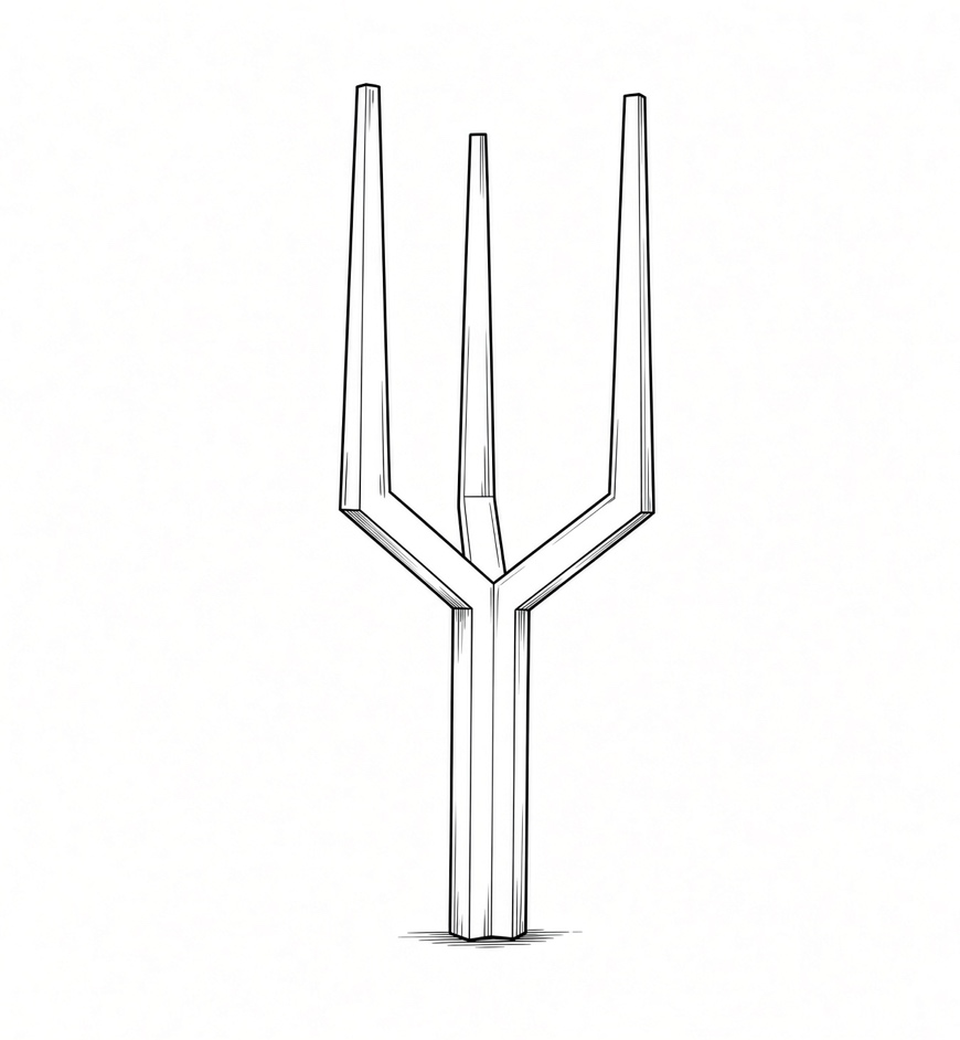
The resonator is excited mechanically - by striking the main radial radiator - or by non-contact methods described in Chapter N1/13. The monolithic structure ensures that vibration transfer between the arms and the waveguide is not interrupted by an interface.
Suitable materials include metals and alloys with low internal damping, particularly aerospace-grade aluminum alloys, titanium, bell bronze, and fused quartz. Resonators made of wood, copper, crystal, or polymers can also be produced and exhibit different acoustic behavior; their placement within the material map is addressed in Chapter N1/15.
Resonators can be manufactured by casting, milling, or additive manufacturing. The selected process affects the achievable angular tolerances and resonance quality, which is itself a subject of study (see N1/06.5). A detailed description of the resonator components is provided in Chapter N1/07 - Normative Terminology.
3.2 FORKER - electromagnetic vibration exciter
FORKER is the project designation for an electromechanical vibration exciter mechanically coupled to the resonator handle, transferring vibration into the entire monolith.
The reference implementation was developed from a loudspeaker voice coil with the diaphragm and enclosure removed; the resonator handle is inserted into the coil former through a compliant coupling. Functionally, it converts an electrical signal into mechanical vibration of the handle, which then acts as a waveguide to the central node and from there to the arms.
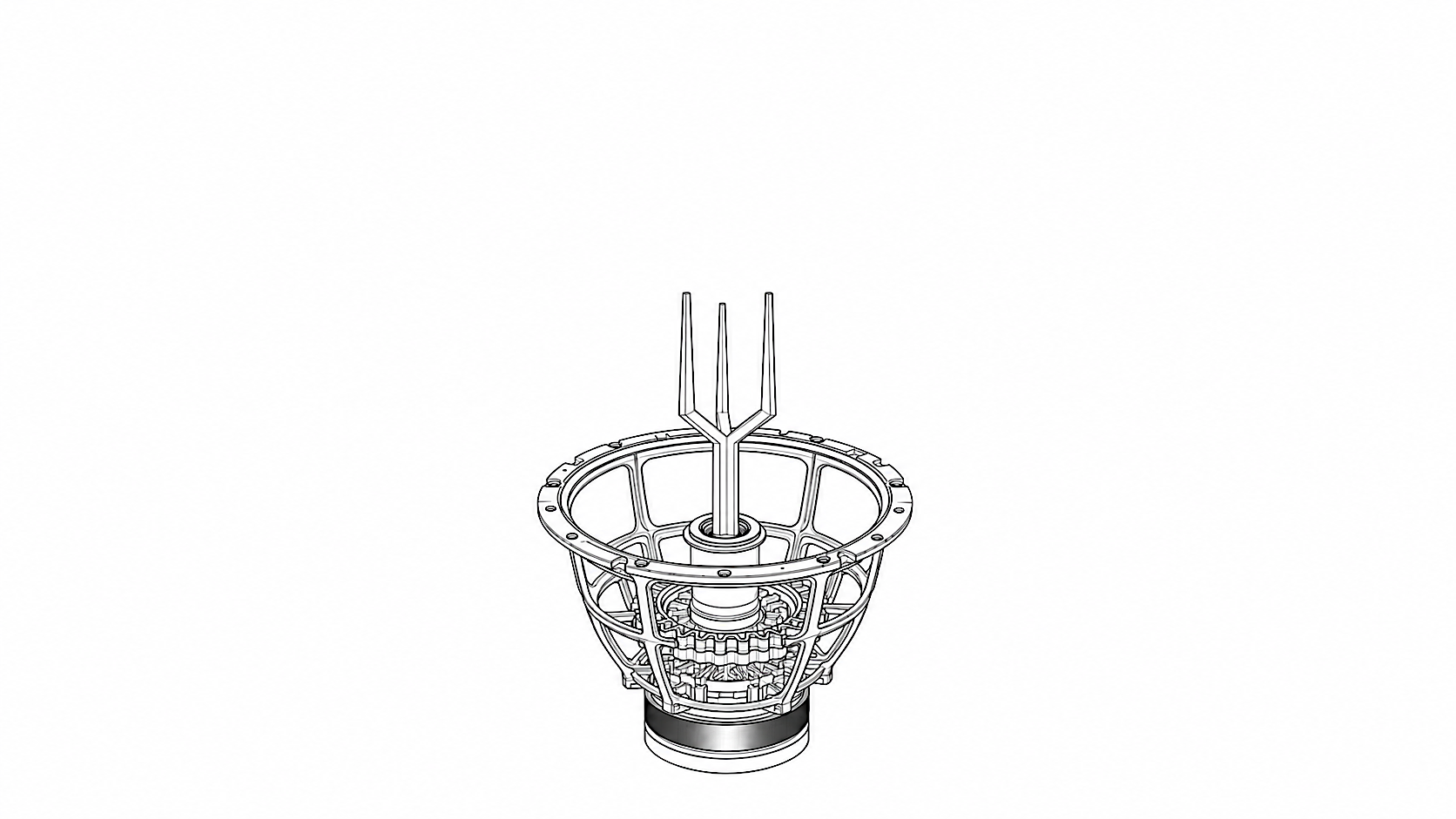
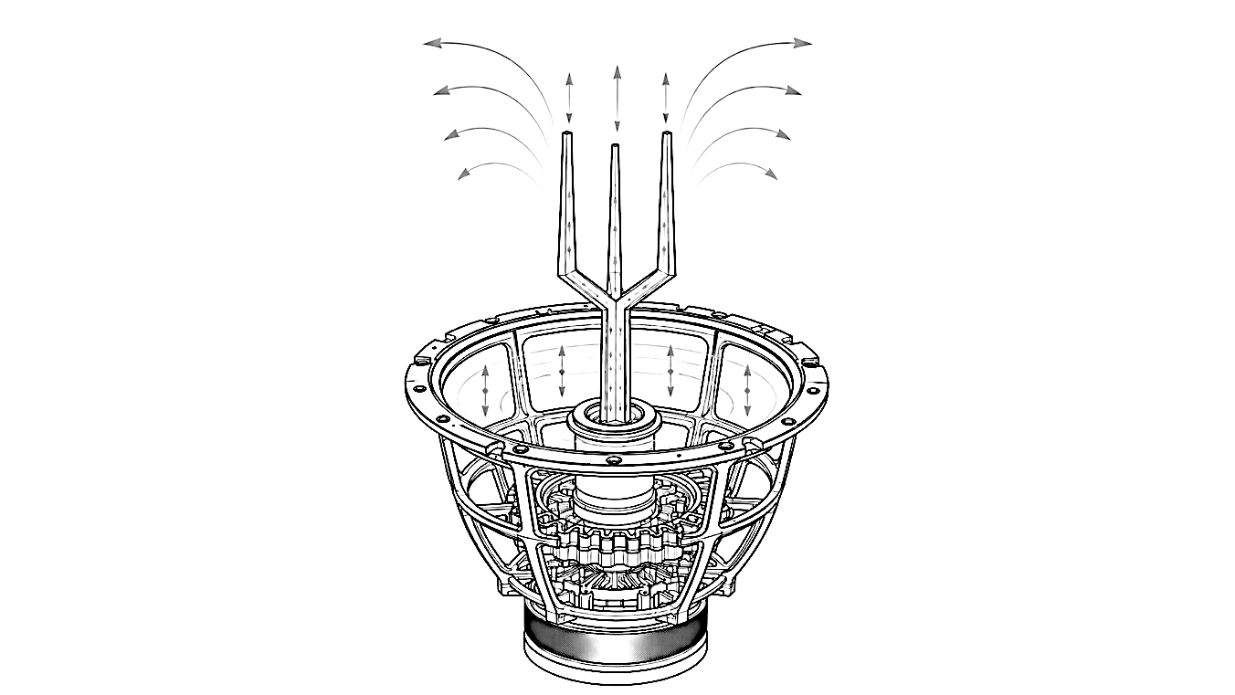
The practical consequence is fundamental. Any frequency within the audible range can be delivered to the resonator at a defined amplitude from an audio amplifier or oscillator - instead of relying on a single, non-reproducible hammer strike. The non-reproducibility of a strike is one of the main methodological weaknesses of the conventional approach: amplitude, point of energy input, and damping caused by contact all vary.
For FORKER to be describable and reproducible, the following parameters must be specified: stiffness and damping of the compliant coupling, mass of the attached assembly, transfer function across the operating band, and maximum amplitude before distortion begins. Phase loss during transfer is not assumed to be zero - it is quantified by measurement.
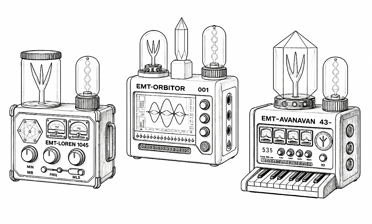
3.3 EMT - Electro-Magnetic Triaural Transductor
EMT is the complete device consisting of a Triaural resonator, FORKER, and drive electronics. It is the lowest level at which the field is controlled: frequency, amplitude, waveform, and duration are adjustable and recordable quantities.
The difference from a passive resonator can be summarized in one sentence. A passive monolith responds to an impulse at its natural resonance and then rings down; EMT can maintain a forced state for an arbitrary duration. The resonator's natural frequency is characteristically associated with a longer ring-down than other frequencies.
This leads to a methodological consequence that applies throughout the corpus: both pulsed and continuous exposure become possible only at the EMT level. Without it, nothing requiring exposure longer than the ring-down can be investigated.
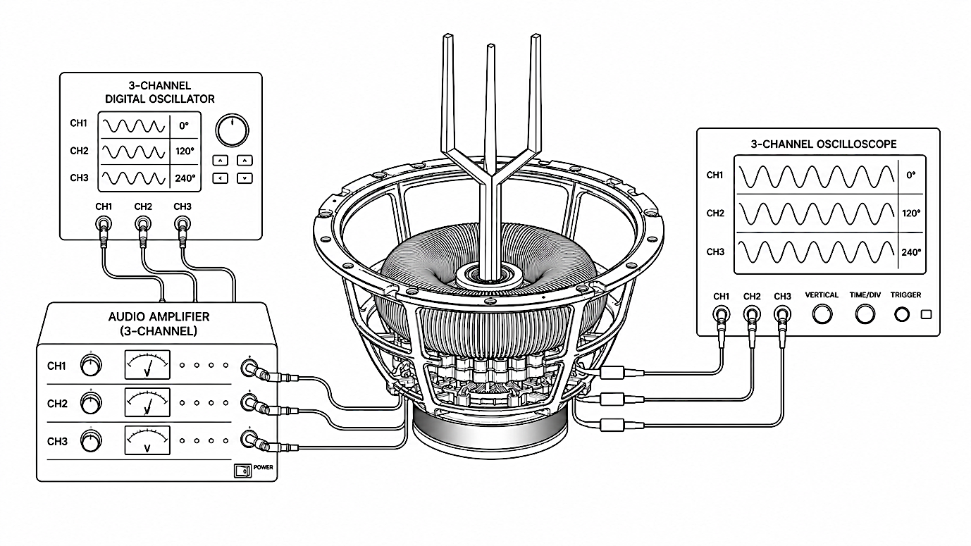
The device operates in three excitation modes. In audio-resonant mode, an amplified audio signal is supplied and the resonator is excited mechanically. In oscillator mode, a signal from a generator is supplied, enabling operation below the audible range within the technical limits of FORKER. In the antenna implementation, the resonator is driven directly from an electromagnetic generator, either passively through a coil or actively by direct contact with the resonator body; this mode is addressed in Document N2.
The reference implementation is EMT - LOREN 1045, where 1045 denotes the natural frequency of the Triaural resonator, equal to 1045 Hz.
3.4 Focal region and its theoretical definition
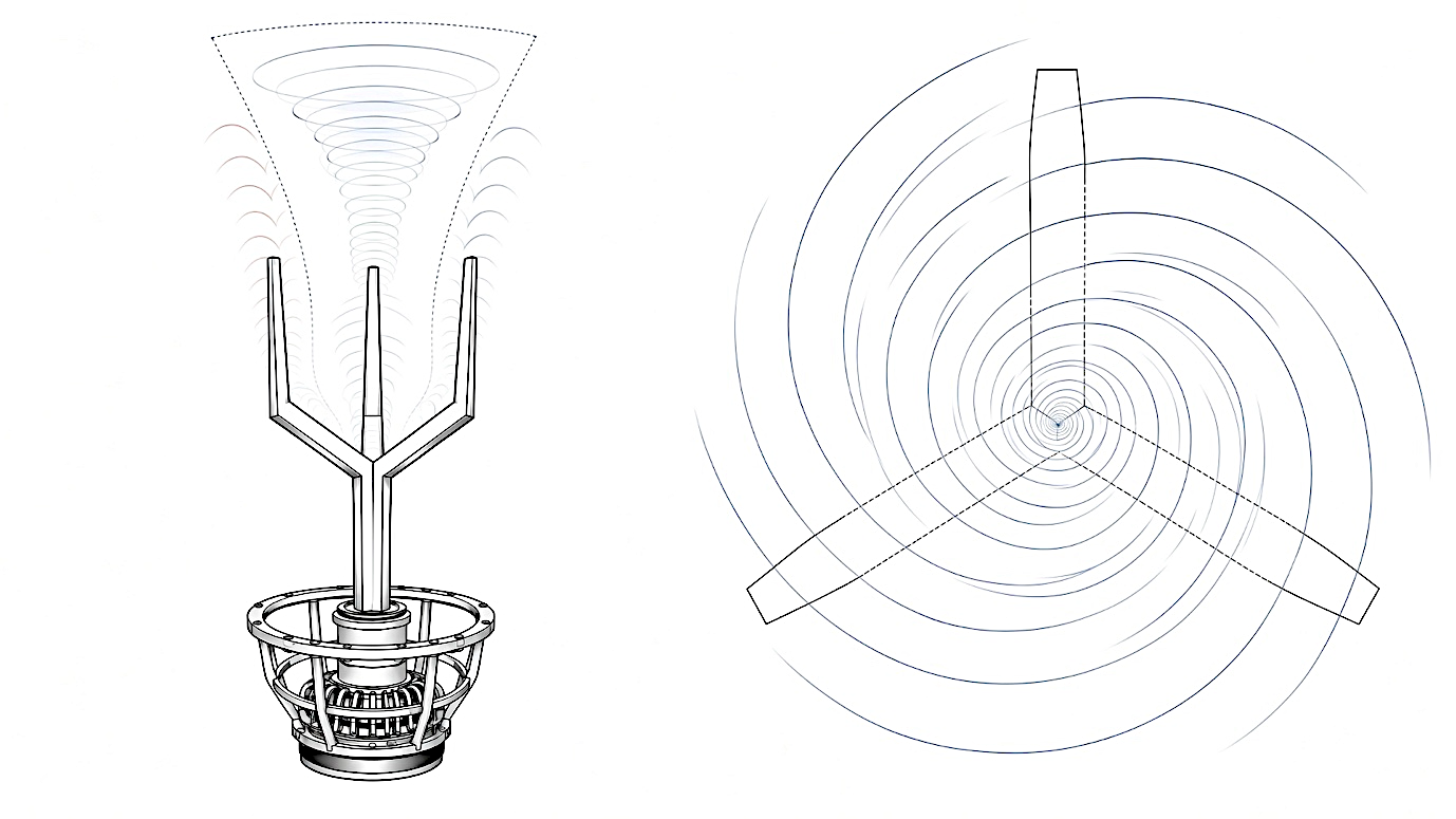
In this document, the focal region is defined as the volume above the central node, bounded by the positions of the main radial radiators, where waves from the individual arms overlap. It is not a point but a volume, and its dimensions depend on geometry and frequency.
3.5 What the system includes and excludes
The term Triaural system includes the resonator, excitation element, drive electronics, and measurement setup. It does not include end-use applications or the environment in which the device is used - those are addressed in Document N3.
COMPLEXITY LADDER L0 - L7
Eight levels lead from a single tuning fork to a spatial chamber. The order is not arbitrary: each level serves as a control for the next, and if any level were skipped, the result at a higher level could not be interpreted.
4.1 Principle of the ladder
The complexity ladder is a reference axis for the entire publication series. It divides the path from a single resonator to a spatial multiresonant chamber and defines the order in which the levels are approached.
The purpose is not to organize the work by difficulty, although difficulty does increase. The purpose is for each level to serve as a control for the next. If a level is skipped, the result at the higher level cannot be interpreted because there is no valid comparison point.
The ladder also determines where each question is addressed within the corpus. The lower half is acoustic and belongs to this document; the upper half extends into Documents N2 and N3.
4.2 Overview of the levels
| Level | Setup | Domain | Document |
| L0 | Passive monolith, mechanical impulse | acoustics | N1 |
| L1 | EMT - monolith with controlled excitation through FORKER | acoustics | N1 |
| L2 | Triangular EMT array aimed at a common focal region | acoustics | N1 |
| L3 | Loudspeakers in a triangular array aimed at a common focal region | acoustics | N1 |
| L4 | AURISONIC mini - spatial array up to 30 cm | acoustics | N1 → N3 |
| L5 | Human-scale AURISONIC | acoustics | N3 |
| L6 | Antenna and coil fields in the same geometry | electromagnetism | N2 → N3 |
| L7 | Hybrid field - acoustics and electromagnetism simultaneously | hybrid | N3 |
4.3 Acoustic branch: L0 through L5
L0 - passive monolith
A resonator without any excitation device, excited by a mechanical impulse. Natural frequency, mode shapes, ring-down, and quality factor are measured - in other words, how long the body continues to ring. This is the baseline state against which everything else is compared, and the only level at which the behavior of the body itself can be determined without the influence of attached mass.
L1 - EMT
One monolith with controlled excitation through FORKER. From this level onward, frequency, amplitude, and duration are adjustable quantities, allowing the response to a defined input to be measured and repeated. Attaching the exciter changes the mass and damping of the system, however, so comparison with L0 is always performed and the difference is recorded.
L2 - triangular EMT array
Three monoliths aimed at a common focal region and driven with controlled phases. This is the first level at which the field arises from the interaction of multiple bodies, and also the first at which it can be tested whether phase control affects the field structure as predicted by calculation.
L3 - loudspeakers in a triangular array
The same spatial geometry, but with conventional loudspeakers instead of monoliths. This level is not a simplification of the previous one - it is its control, and it has a special status throughout this document. It is discussed in Section 4.5.
L4 - AURISONIC mini
A spatial source array up to approximately thirty centimeters in size, with a rhombicuboctahedral frame. This is the first level at which the field is formed in three dimensions rather than in a plane. It is used to validate metrics and procedures before proceeding to a human-scale structure.
L5 - human-scale AURISONIC
The same arrangement enlarged enough to accommodate a person. This level belongs to Document N3 together with all ethical and safety requirements arising from human presence.
4.4 Electromagnetic and hybrid branch: L6 and L7
L6 - electromagnetic upgrade
The same geometry implemented as an antenna array or coil field. It is addressed in Document N2. It appears in the ladder only after the acoustic branch because acoustic measurements are less expensive, faster, and safer, and provide an initial basis for understanding what the geometry may contribute.
L7 - hybrid field
Acoustic and electromagnetic excitation acting simultaneously on the same setup. This is the highest level of the ladder. It is investigated only after the two domains have been independently verified, because otherwise their respective contributions to the result could not be separated.
4.5 L2 versus L3 - the key control
The comparison between the second and third levels is the single most important measurement in the entire N1 program, and it is worth explaining why.
Three monoliths and three loudspeakers are placed in identical geometry, driven at the same frequency, and adjusted to produce the same acoustic pressure in the focal region. The field structures are then compared.
If the fields cannot be distinguished, the observed field properties follow from the arrangement and phase relationship of the sources alone. In that case, the Triaural field could also be realized using three phase-controlled sources, which is standard phased-array acoustics.
If the fields differ reproducibly, this will show that replacing the monolithic resonators with conventional sources changes the measured field structure. The next question will be which property of the monoliths causes the difference and whether it is related to the degenerate pair described in Chapter N1/09.
The outcome of the L2 versus L3 comparison determines what role can be attributed to the monolithic resonators in subsequent research. If no measurable difference is demonstrated between the arrays in the observed field properties, those properties should, within that experimental arrangement, be explained primarily by source geometry and phase relationships. If a difference is demonstrated, the question of its origin and its relationship to the modal structure of the monoliths is opened. The result of this control therefore affects the interpretation of hypotheses that invoke a specific contribution from the monolithic resonator; their explicit links to the individual ladder levels are listed in Chapter N1/22.
The decision gate applies to a specific hypothesis, not to an entire research direction. A negative result closes the claim that was tested and is not by itself a reason to terminate a related branch if that branch rests on a different mechanism. The decision to continue or stop is recorded with justification and does not follow automatically from the result. In this way, the document guards against two opposite errors at once: continuing despite a falsified claim, and closing a branch on the basis of an assumption without the full context.
4.6 Why the order is maintained
Skipping a level does not save time; it only moves uncertainty forward. If, for example, a human-scale chamber were built without first performing the L2 versus L3 comparison, any measured effect would have two equally plausible explanations, and distinguishing between them would require going back down four levels afterward.
The sequence also protects the budget. Each level is an order of magnitude more expensive than the previous one, and the decision to continue is made only after the result of the preceding level is known. The ladder is therefore both a methodological tool and a sequence of decision points.
Assignment of levels to timeline phases:
| Level | Phase | Cost note |
| L0 - L1 | F0 | sample manufacturing and baseline measurement; lowest-cost ladder item |
| L2 - L3 | F0 and F1 | key comparison under Chapter N1/04.5; requires three sources and positioning |
| L4 - L5 | F1 and F2 | visualization, liquid media, optics, and high-speed recording |
| L6 - L7 | outside N1 scope | electromagnetic branch; addressed in Documents N2 and N3 |
Costs in this document are not divided by ladder level, but by equipment items in Chapter N1/19.3. A second parallel classification would diverge after the first change and one of the two would become obsolete. The link between a level and its cost is therefore maintained through the phase structure: Chapter N1/21.8 specifies which items are acquired in each phase.
DEVICE CLASSIFICATION
Triaural geometry can be used in two ways: for sound and for electromagnetic fields. This chapter separates the two and defines how they differ.
5.1 Acoustic monolithic resonators
These are monolithic bodies consisting of a waveguide and a set of resonant arms. They are excited mechanically or through FORKER and produce an acoustic field around the focal region.
The hypothesized result of excitation is the formation of a rotating component of the field in the focal region - a structure that does not simply repeat in space as a standing wave, but also carries circulating phase structure. This claim is Hypothesis H-N1-01 and is nowhere presented in this document as documented. The physical rationale and falsification criterion are given in Chapter N1/09.
The resonator transfers acoustic energy along two paths: through the air into the surroundings and mechanically through the handle into whatever it contacts. The two paths are measured separately because conflating them can lead to incorrect conclusions (see N1/14 and N1/18).
5.2 Multipolar electromagnetic devices
The same geometry can be implemented in conductive material and driven by an electromagnetic signal. In that case, it functions as an antenna with three or more arms extending from a central node.
Candidate materials include highly conductive metals, semiconductors, piezoelectric crystals, and carbon-based composites. Construction methods include casting, milling, additive manufacturing, or conductive joining of individual segments in the prescribed spatial geometry.
Questions concerning radiation pattern, near field, and coupling between topologies are addressed in Document N2 and are not examined here. Document N1 primarily establishes the geometry and terminology adopted by N2.
5.3 Hybrid devices
A hybrid device is a setup in which acoustic and electromagnetic excitation are applied simultaneously to the same body. Such an arrangement is classified as Level L7 of the complexity ladder and is investigated only after the two domains have been independently verified.
GEOMETRIC DESCRIPTION
This chapter defines the resonator shapes distinguished in the program and the criteria used to distinguish them. The key parameter is angle, and it will become clear that angle is also the quantity that must be measured most precisely.
The geometric description of the resonator is divided into several levels in this document. The number of arms n determines the basic topology. The vertex angle φ and the derived inclination θ determine the spatial arrangement of the support arms. A separate angle β defines the orientation of the main radial radiators relative to the central body axis.
The next level consists of articulations, segment lengths, cross-sections, and other dimensions. These parameters are described separately so that a change in one geometric property is not confused with a change in another.
6.1 What defines a configuration
The spatial arrangement of the resonator is defined by two basic quantities: the number of main radial radiators and the vertex angle between two adjacent support arms. Let these be denoted n and φ.
The number of arms determines the central segment angle - the angular spacing between arms when viewed from above - as 360° divided by n. For three arms the result is 120°, for four arms 90°, and so on according to the table in Chapter N1/08, item A.
The angle φ is the vertex angle between the axes of two adjacent support arms. For a given number of arms, it determines the support-arm inclination relative to the central body axis, denoted θ. For φ values below 120°, two mirror orientations of this inclination exist, as described in Section 6.4.
The two quantities are geometrically linked, and for a known n the basic configuration can be defined using either φ or θ. This document uses φ as the primary parameter for a practical reason: the vertex angle between the support arms can be determined directly from the resonator geometry, whereas θ is referenced to the central body axis.
The pair n and φ defines the basic opening of the support arms. To determine their spatial orientation unambiguously, the base or mirror branch defined in Section 6.4 must also be specified. These parameters do not, however, define the complete resonator geometry. The main radial radiators may be parallel, convergent, or divergent relative to the central body axis, and this relationship is described separately by the angular parameter β in Section 6.5. Additional parameters - segment lengths, cross-sections, articulations, and their angles - are added to the base configuration as further geometric degrees of freedom.
6.2 Relationship between the support-arm vertex angle and axial inclination
Let θ denote the angle between the central body axis of the resonator and the axis of a support arm, and let φ denote the vertex angle between the axes of two adjacent support arms. For n arms distributed uniformly around the body axis, the following relationship applies:
cos φ = cos²θ + sin²θ · cos (360°/n)
For three arms, the expression simplifies to:
cos φ = ( 3 cos²θ − 1 )/2
Conversely, for a specified angle between the arms, the inclination is calculated as:
cos θ = √ ( ( 2 cos φ + 1 )/3 )
The angle θ corresponds to the upper support-arm inclination (HSNR). In configurations where the main radial radiators are parallel to the central body axis, their direction is not included in the calculation of φ and θ; only the support-arm geometry is relevant.
Because the relationship contains cos^2θ there are two axial orientations of the support arms for φ values below 120°. The values θ and 180^∘-θ form mirror configurations with the same vertex angle φ. Between the two branches lies the EQUATORconfiguration, in which θ = 90° and the support arms lie in a plane perpendicular to the central body axis.
The privileged configurations listed below represent the base branch from TETRATIP through EQUATOR. Their mirror equivalents form the second branch of the same geometric family and may be examined in separate comparative measurements.
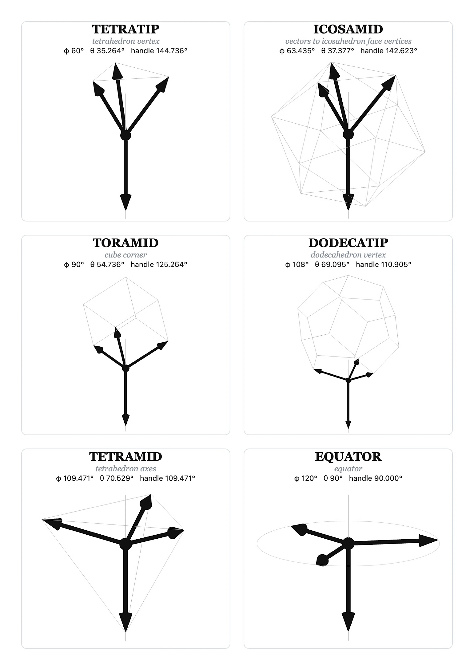
| Configuration | Vertex Angle φ | Inclination θ (HSNR) | Angle to Handle (DSNR) | Geometric Reference |
| TETRATIP | 60° | 35,264° | 144,736° | tetrahedron vertex |
| ICOSAMID | 63,435° | 37,377° | 142,623° | radial vectors to vertices of an icosahedral face |
| TORAMID | 90° | 54,736° | 125,264° | cube corner |
| DODECATIP | 108° | 69,095° | 110,905° | dodecahedron vertex |
| TETRAMID | 109,471° | 70,529° | 109,471° | regular tetrahedron |
| EQUATOR | 120° | 90° | 90° | equatorial plane |
The table lists six reference points of the continuous C3 geometric family. The first five configurations are derived from distinct symmetric spatial arrangements; EQUATOR represents the boundary condition in which the support arms lie in a plane perpendicular to the central body axis. In the TETRAMID configuration, the vertex angle between the support arms also equals the angle between a support arm and the handle. The direction of the central waveguide and the three support-arm directions therefore form four geometrically equivalent directions of a regular tetrahedron.
6.3 Six basic configurations
The following six configurations form the initial set of support-arm geometries on which the first measurements are based. Their selection follows geometrically privileged directions derived from regular three-dimensional forms and from a special equatorial state. The illustrated solids indicate the geometric origin of the corresponding directions; they are not part of the resonator.
TETRATIP - 60°
The support arms form a vertex angle of 60° and are inclined by 35.264° from the central body axis. Their directions correspond to three edges extending from one vertex of a regular tetrahedron. This is the narrowest of the privileged configurations on the base branch.
With main radial radiators parallel to the body axis, these radiators remain closest to the axis among all six configurations. The effect of this geometry on the position, extent, and structure of the resulting field is a subject of measurement.
ICOSAMID - 63.435°
The support arms form an angle of approximately 63.435° and are inclined by 37.377° from the central body axis. The configuration is derived from three radial vectors extending from the center of a regular icosahedron to the three vertices of one triangular face.
ICOSAMID is geometrically close to TETRATIP, but its angle has a different origin in icosahedral symmetry. This proximity makes it a useful comparison point for studying the sensitivity of modal structure and field behavior to small, geometrically motivated changes in angle.
TORAMID - 90°
The support arms are mutually orthogonal and are inclined by 54.736° from the central body axis. Their directions correspond to three edges of a cube extending from one vertex, while the central waveguide lies along the corresponding body diagonal.
The three mutually orthogonal directions provide a natural orthogonal geometric frame for resolving measured quantities into spatial components. The name TORAMID is the historical designation of the configuration and is not derived from cube geometry; the cube corner serves only as its geometric reference.
DODECATIP - 108°
The support arms form an angle of 108° and are inclined by 69.095° from the central body axis. The configuration is derived from three equivalent directions extending from one vertex of a regular dodecahedron.
The value 108° lies very close to the tetrahedral angle of TETRAMID, although the two configurations have different geometric origins. This pair therefore provides another natural comparison point for investigating whether small differences between two privileged angles produce measurable differences in modal structure or in the resulting field.
TETRAMID - 109.47°
The support arms form the tetrahedral angle, whose exact value is arccos(−1/3), or 109.4712°. They are inclined by 70.529° from the central body axis.
The direction of the central waveguide and the directions of the three support arms form four geometrically equivalent directions, with the same angle between every pair. The arrangement therefore corresponds to directions from the center of a regular tetrahedron to its four vertices.
The same tetrahedral angle also occurs in the bonding geometry of carbon in an sp³ arrangement and in silicon-oxygen tetrahedra. The possible significance of this geometric correspondence for material-related questions is treated as a hypothesis in Chapter N1/15.
EQUATOR - 120°
The support arms form an angle of 120°, and their axes lie in a single plane perpendicular to the central body axis of the resonator. Both the inclination θ and the angle between a support arm and the handle are 90°.
EQUATOR is the boundary point between the two mirror branches of the C3 geometric family. Passing through this configuration reverses the axial orientation of the support arms relative to the direction of the central waveguide.
The special status of this configuration leads to a separate experimental question: whether the perpendicular connection of the support arms to the central-waveguide direction changes the transfer of mechanical energy through the central node and the amount of vibration transmitted into the handle. This expectation is not treated in the document as a geometric consequence and requires modal analysis and experimental verification.
6.4 Mirror configurations and axial polarity
Every privileged configuration with φ < 120° has a mirror geometric equivalent with the same vertex angle. Its corresponding inclination is 180^∘-θ, with the support arms passing to the opposite side of the plane perpendicular to the central body axis.
A mirror configuration is not spatially identical to the original configuration because the central waveguide defines an oriented axial direction of the resonator. The two configurations may therefore have different mechanical conditions at the central node despite having the same vertex angle φ.
EQUATOR is the common boundary point of both branches. A systematic comparison of the original and mirror configurations is treated as a separate research question. The related hypothesis is H-N1-59.
6.5 Orientation of the main radial radiators
The geometry of the support arms and the geometry of the main radial radiators represent two distinct degrees of freedom. Values φ and θ define the direction of the support arms from the central resonant node to the articulation nodes. The direction of the main radial radiator from the articulation node to its free end is described separately.
This document introduces the signed parameter β, which describes the radial inclination of the main radial radiator axis relative to the central body axis of the resonator. The radiator direction is evaluated from the articulation node toward its free end.
The following sign convention is used for β:
β = 0° - the main radial radiator is parallel to the central body axis.
β > 0° - the radiator moves away from the axis toward its free end; this is a divergent configuration.
β < 0° - the radiator approaches the axis toward its free end; this is a convergent configuration.
The sign of β determines the radial orientation of the radiator, while the absolute value |β| gives the magnitude of its deviation from the parallel arrangement.
In a symmetric Triaural resonator, all three main radial radiators have the same β value and their directions repeat rotationally every 120°. The value of β does not change the vertex angle φ or the support-arm inclination θ; it changes the geometry only beyond the articulation node. Two bodies can therefore have the same n, φ, and θ but different β values and represent geometrically distinct resonators.
Changing β alters the relative positions of the free ends of the main radial radiators, their distance from the central axis, and the geometric definition of the region above the central node. Its effect on modal structure, arm-to-arm coupling, focal-region position, and spatial field distribution cannot be determined from geometry alone and is the subject of separate computational and experimental comparison.
Three classes are distinguished in the basic notation:
PARALLEL - β = 0°
CONVERGENT - β < 0°
DIVERGENT - β > 0°
When a complete geometric specification is required, the β value is appended to the configuration name, for example TORAMID β+15°, TETRAMID β0°, or EQUATOR β−10°.
The complete basic geometric notation of a Triaural resonator can therefore be expressed as the sequence
n→(φθ)→β→(a_i)→(d_ip_i),
where n specifies the number of arms, φ and θ define the support-arm geometry, β defines the basic orientation of the main radial radiator, (a_i) its optional articulation angles, and (d_ip_i) the lengths and cross-sections of the individual segments.
6.6 Configurations with a higher number of arms
The relationships above apply to any number of arms. With four arms, the central angle decreases to 90°, and for each φ value there is a corresponding inclination θ according to the general relationship in Section 6.2.
A four-arm arrangement also allows a configuration in which the arms point toward the vertices of a regular tetrahedron while the handle extends from the center. Such an implementation has a different symmetry from the three-arm version and is introduced in Chapter N1/09 as a separate question.
For more than four arms, the procedure remains the same. The practical limit is set by manufacturing constraints and the mutual spacing of the arms at a given cross-sectional thickness.
The parameter β describes the overall direction of the main radial radiator regardless of any additional bends. The suffixes -CUSP and -FLARE are used only for articulation-induced changes of direction along the radiator and do not replace the β specification.
6.7 Articulated variants
The main radial radiator may bend at articulation nodes as defined in Chapter N1/07, item G. The bend is a property of the configuration and is appended to its name as a suffix.
The suffix -CUSP denotes a bend toward the body axis, or inward. This produces configurations such as TETRATIP-CUSP, TORAMID-CUSP, or TETRAMID-CUSP. An inward bend brings the arm tips closer to the axis and changes the position and shape of the focal region.
The suffix -FLARE denotes a bend away from the axis, or outward. The tips move farther apart and the focal region expands.
The base configuration remains unambiguously defined in this notation, while articulation is an additional modifier. For multiple bends, the number of articulations and articulation angles are specified according to Chapter N1/08, item G.
6.8 Geometric tolerance
The precision with which the angles must be maintained remains an open question, and its answer will affect the entire subsequent course of Program N1.
The reason follows from Chapter N1/09. A rotating state arises from the superposition of two mode shapes with the same frequency; deviation from symmetry separates those frequencies and the rotation settles into a standing pattern. The decisive quantity is therefore the splitting of the degenerate pair, denoted Δf.
The tolerance study uses a series of samples with controlled angular deviations of 0°, 0.5°, 1°, 2°, and 5°. For each sample, Δf is measured together with the amplitude of the rotating component. The result is a curve of Δf as a function of deviation, which can be compared with the prediction of the computational model described in Chapter N1/17.
The answer directly affects both budget and manufacturing technology. If the phenomenon survives a ±5° deviation, manufacturing is accessible and independent replication is realistic. If it requires ±0.1°, precision machining and metrology become a central focus of Program N1.
A curve has one additional advantage over a single data point: a continuous relationship can be compared with the model point by point, providing stronger evidence than a one-time observation. The relevant hypotheses are H-N1-26 and H-N1-51.
6.9 Open taxonomy
The listed configurations form an initial set selected for clarity and for their links to basic spatial arrangements. The set remains open, and additional geometrically meaningful classes may be added.
The taxonomy may include, in particular, asymmetric configurations with unequal angles between arms, helical arms with geometry varying along their length, multilayer arrangements with arms at several levels, and mutually interwoven arms in helical or braided forms as described in Chapter N1/07, item F.
The six basic configurations in Section 6.3 represent reference points of the continuous C3 geometric family. An open experimental question is whether the geometrically privileged points of this family also exhibit distinct or mutually distinguishable physical properties; this question is captured by Hypothesis H-N1-25.
A separate open branch is the complete C3 geometric taxonomy of directions derived from regular and other symmetric polyhedra. A systematic treatment would exceed the scope of this chapter and is suitable for a separate theoretical study or an independent research team.
NORMATIVE TERMINOLOGY
The following terminology is binding throughout the corpus. Without it, meaningful statements about measurement are not possible. If two people say “arm” but each means something different, their results cannot be compared.
To define TRIAURAL precisely as a whole and harmonize terminology for cooperative research, the individual segments, components, and geometric relationships require unambiguous names. The following terms are used throughout Documents N1, N2, and N3 exclusively in the meanings defined below.
7.1 Field types
A scalar field assigns one number without direction to every point in space and time; typical examples are temperature, pressure, or electric potential. A vector field assigns both magnitude and direction, such as particle velocity or electric field strength. A tensor field assigns a set of mutually related components, as required, for example, when describing stress in a solid body.
Acoustic pressure is a scalar field. Particle velocity is a vector field and, in a linear potential description, can be expressed as the gradient of a scalar velocity potential.
This leads to a condition that is fundamental to Program N1: the curl of a gradient is identically zero, so the particle-velocity field is irrotational in this approximation. The document therefore does not use the term acoustic vortex to mean local vorticity of particle velocity. Instead, it refers to the phase structure of the wave field, which may contain a phase singularity and carry orbital angular momentum, as documented in the peer-reviewed literature on acoustic vortices. These phenomena are discussed in Chapter N1/09.5.
To avoid confusion, five quantities must be distinguished:
- Acoustic pressure is a scalar field; the concept of curl does not apply directly to it.
- Particle velocity, in the linear potential approximation, is the gradient of a scalar potential, so its curl is zero.
- A phase singularity is a location where the complex pressure amplitude approaches zero and phase is undefined; its existence does not contradict zero curl of the particle-velocity field.
- Orbital angular momentum is a property of the wave field associated with its spatial, particularly azimuthal, phase structure; it cannot be equated with local vorticity of particle velocity [14].
- Acoustic streaming is a nonlinear second-order phenomenon. Its time-averaged velocity field may carry circulation and represents a mechanism distinct from the linear oscillation of the acoustic field [15, 16].
Zero curl of the particle-velocity field in the linear potential description therefore does not exclude a phase singularity or orbital angular momentum. Statements in this document concerning a “rotating component” refer, in this sense, to these properties of the wave field; acoustic streaming is evaluated separately as a possible nonlinear mechanism.
7.2 Resonator segments and components
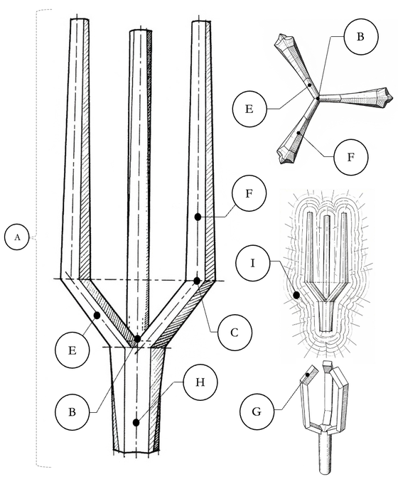
A) RESONATOR BODY
The body means the entire monolithic or modular object in the specific geometry defined by the geometric description in Chapter N1/06.
B) CENTRAL RESONANT NODE
The common connection point of the central waveguide and the support arms of the resonator. Mechanical coupling of the individual segments and transfer of vibration between them occur at this node. Its modal behavior, amplitude relationships, and phase relationships are subjects of computational and experimental analysis.
C) ARTICULATION NODE
The junction between a support arm and a main radial radiator, or between individual articulations of a main radial radiator - for example, when the main radial radiator is bent and therefore divided into several smaller segments at articulation angles.
D) SEGMENT
Any continuous part of the whole. This may be a support arm, a main radial radiator, or an articulation.
E) SUPPORT ARM
A segment connecting the central resonant node to the main radial radiator, or a section connecting the central node to a subsequent articulation of the main radial radiator. Its cross-section is generally identical to that of the main radial radiator, although this is not required. The length and inclination of the support arm determine the position of the articulation node relative to the resonator's central axis. The subsequent spatial orientation of the main radial radiator is defined by parameter β according to Chapter N1/06.5. The support arm may connect to the main radial radiator at an acute or obtuse angle, or it may have a curved shape.
F) MAIN RADIAL RADIATOR
The primary vibrating segment of a resonator arm. In mechanically excited acoustic resonators, it may serve as the point of direct impact or other excitation. Its length, cross-section, material, and geometry significantly influence the modal properties of the resonator; the resulting natural frequencies, however, depend on the mechanical behavior of the entire coupled structure. The cross-section is typically square, circular, or triangular, but it may take the form of any planar geometric shape. The main radial radiator may vary in geometry along its length, for example as a helix or with variable diameter. Individual main radial radiators may be mutually parallel or interwoven in space without contact; they may converge or diverge. Their mutual geometric relationship may take the form of a segmented helix, an interwoven polygonal chain, a zig-zag helix, any braided structure, or combinations of these. Its basic orientation relative to the central body axis is defined by parameter β according to Chapter N1/06.5.
G) ARTICULATIONS OF THE MAIN RADIAL RADIATOR
Sections into which the main radial radiator may, but need not, be divided. If it is bent along its length and thereby divided into separate segments - whether within a monolithic body or a modular construction - those segments are called articulations. In regular articulated variants, they may be spaced uniformly and use the same articulation angle, although this is not required by the definition. The number of articulations is unrestricted, and the articulation angles may take arbitrary values.
H) CENTRAL WAVEGUIDE (HANDLE)
The central part of the resonator is used to hold the device in the operator's hand, mount it in a stand, or mechanically connect it to an exciter. In manual use, it also forms the mechanical interface between the resonator body and the operator's body. In all cases, it represents the mechanical path between the central resonant node and the point of holding, mounting, or excitation. The nature of vibration and energy transfer in this segment is addressed in Chapter N1/14.
I) TRIAURAL FIELD
The region around a Triaural resonator in which the spatial distribution of measured physical quantities is observed during excitation. In acoustic measurements, it is primarily the result of superposition of waves associated with vibration of the individual arms. The extent and structure of the field are determined by measurement according to Chapters N1/09 and N1/10.
DEFINITION OF ANGULAR PARAMETERS
Angles are to Program N1 what gear dimensions are to watchmaking. The following definitions specify which angle is measured where - so that two resonators can be compared even if they were made by two different people on two different continents.
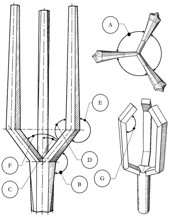
A) CENTRAL SEGMENT ANGLE
The angular spacing of the arms when viewed from above, i.e., the division of the resonator circumference. For three arms it is 120°, for four 90°, for five 72°, for six 60°, for seven 51.4286°, for eight 45°, for nine 40°, for ten 36°, for eleven 32.7273°, and for twelve 30°.
B) LOWER SUPPORT-ARM INCLINATION (DSNR)
The opening angle of the resonator between the central waveguide and the support arm.
C) UPPER SUPPORT-ARM INCLINATION (HSNR)
The opening angle between the resonator's central body axis and the support arm. HSNR = 180° − DSNR.
D) INNER SUPPORT-ARM ARTICULATION ANGLE (VNUANR)
The inner angle formed by the support arm and the main radial radiator. For resonators whose main radial radiators are parallel to the body axis defined by the handle, VNUANR = DSNR.
E) OUTER SUPPORT-ARM ARTICULATION ANGLE (VOUANR)
The outer angle formed by the support arm and the main radial radiator. In the parallel arrangement, VOUANR = HSNR + 180°.
F) SUPPORT-ARM VERTEX ANGLE
The angle formed by two adjacent support arms or their first articulations. If two adjacent support arms were removed from the resonator, they would form a V-shaped object; this angle defines the opening between them.
G) ARTICULATION ANGLES
The bend angles of the main radial radiator at articulation points. They curve the radiator toward or away from the resonator's central axis. The number of articulations is unrestricted, and the articulation angles may take arbitrary values.
The precision with which these angles must be maintained is not yet known. This is a separate research question developed in Chapter N1/06.8 as a tolerance study; its result directly determines the manufacturing technology required by Program N1.
PHYSICAL BASIS
Why should a three-pronged tuning fork behave differently from a two-pronged one? This chapter proceeds step by step: what is known about sound, what follows from that for our geometry, and above all - what measurement could show that we are wrong. It is the most important chapter in the document because everything else rests on it.
9.1 Starting point: what a two-pronged tuning fork does
A conventional tuning fork has two prongs that, in the fundamental bending mode, oscillate symmetrically in opposition. As the prongs open, both free ends move away from the median plane and their transverse reactions at the common base act in opposite directions. These reactions largely cancel at the junction, so only a small transverse component of motion is transmitted into the handle. The handle therefore participates primarily in the longitudinal direction [17].
The consequence is easy to observe: when a sounding tuning fork is slowly rotated about its axis, the measured or perceived sound amplitude at a fixed point changes. Depending on the observation direction, radiation from the two prongs combines with different phase relationships, producing reinforcement in some directions and strong suppression of acoustic pressure in others.
The acoustic radiation of a conventional tuning fork has a characteristic multilobed directivity pattern in the near field, with pronounced minima. As distance increases, the spatial pattern changes and takes on a simpler directional structure in the far field [17]. This behavior is among the conventionally described properties of a two-pronged tuning fork [D].
9.2 What changes with three prongs
Now consider a body with three geometrically equivalent prongs spaced 120° apart. If the prongs are identical in material and geometry, the natural question is which modal classes are permitted by the symmetry of such a body.
Symmetry theory provides the answer. In bodies with threefold rotational symmetry, the relevant nonsymmetric modal class can form a two-dimensional degenerate pair: two linearly independent mode shapes with the same natural frequency that differ in spatial orientation [18].
From the standpoint of symmetry, one can distinguish fully symmetric modes, in which all three prongs behave equivalently, from a nonsymmetric two-dimensional modal class in which a degenerate pair appears. In the simplest symmetric picture, all three prongs deflect simultaneously in the same way, as if the body were "breathing." The nonsymmetric class is described by two mutually independent mode shapes at the same frequency.
This pair is referred to as a degenerate pair.
Symmetry is denoted in the technical literature using standard shorthand. The letter C denotes cyclic rotational symmetry, and the number gives the number of equivalent rotations within one full revolution. C3 symmetry therefore means that the body maps onto itself after a rotation of 120°. Related cases are C2 for a rotation of 180° and C4 for a rotation of 90°.
The symmetry of a body constrains which modal classes can exist even before a specific specimen is manufactured. C2 symmetry alone does not produce an analogous two-dimensional modal class in which degeneracy is enforced by symmetry. A two-pronged tuning fork therefore does not possess the same symmetry-protected modal pair as a three-pronged body with C3 or C3v symmetry.
A more complete designation for an ideally symmetric Triaural resonator is C3v, where the lowercase letter denotes the presence of mirror planes passing through the prongs. In a chiral modification of the body, these planes may disappear, leaving only C3 rotational symmetry.
9.3 Why rotation may arise
If two linearly independent mode shapes exist at the same natural frequency, they can be combined linearly. If both components are excited with an appropriate amplitude ratio and a relative phase shift of approximately 90°, the resulting superposition can form a spatially rotating deformation pattern. The mere existence of a degenerate pair, however, does not determine which specific combination of modes will actually be produced by a given excitation method.
A useful mathematical analogy is provided by a three-phase electric motor. Three coils spaced 120° apart and driven by signals with the appropriate phase offsets create a rotating magnetic field. The coil assembly itself does not rotate mechanically; the spatial field pattern rotates. The analogy illustrates a phase-progressing superposition and is not evidence of the same physical mechanism in the resonator.
If oscillation of the three prongs were to establish a stable cyclic phase progression of approximately 0°, 120°, and 240°, a spatially progressing phase structure around the Triaural axis could be expected. Whether such a state arises spontaneously under impulsive or in-phase excitation of a particular resonator is an experimental question captured by hypothesis H-N1-01.
Two numbers describing the same state
At this point, two different phase offsets appear in the text and must be distinguished, because confusing them would lead to an incorrect conclusion.
In an ideal two-dimensional modal subspace, the same phase-progressing state can be described either by three spatially distributed components with a cyclic 120° offset, or by two independent modal coordinates in quadrature, with a 90° offset.
The reason there are two modes rather than three follows from the structure of the relevant nonsymmetric modal class. The three prong-amplitude components do not represent three independent degrees of freedom; the state can be fully described by two independent modal coordinates.
A rotating state in such a two-dimensional space can be formed by combining two independent components in quadrature, that is, with a 90° phase shift. This is the same mathematics as the parametric description of a circle, where one coordinate follows the cosine and the other the sine.
The conversion between these two descriptions has a standard form in electrical engineering: the Clarke transformation, also known as the αβ transformation [19]. It converts a three-component abc system into two orthogonal coordinates, α and β. In a balanced sinusoidal three-phase system with 120° phase separation, the resulting α and β components form a quadrature pair and describe the same rotating vector in a two-dimensional plane. In electric motor control, this is a standard mathematical tool.
The Clarke transformation is used here as a mathematical analogy for conversion between three-component and two-component descriptions; it is not a claim that the mechanical modes of the resonator are identical to an electrical three-phase system. These are two mathematically equivalent descriptions of the same ideal phase-progressing state.
Because the relevant modal subspace has two independent degrees of freedom, its state can in principle be reconstructed from two independent and appropriately positioned sensing channels. A third channel provides redundant information useful for checking consistency, symmetry, and measurement error; this is why the three-channel magnetic pickup in Chapter N1/13.3 is designed in this way.
Vibration theory therefore permits the existence of a rotating superposition within a degenerate pair. Experiment must separately determine whether a particular resonator actually possesses such a pair, whether the selected excitation method excites it with the required amplitude and phase relationship, and whether the resulting state remains stable or mixes with symmetric and other modal components.
9.4 The condition that holds it all together
A rotating superposition is simplest and most stable when both members of the degenerate pair have the same natural frequency. If degeneracy is broken and the modal frequencies separate by Δf, their relative phase begins to evolve over time. A pure rotating state may therefore cease to be stationary and can transition into a pulsating, standing, or hybrid modal superposition.
The magnitude of this effect depends on the splitting Δf, the quality factors of the individual modes, their damping, the excitation method, and the observation time. There is therefore no universal threshold at which an arbitrarily small splitting automatically eliminates the rotating component; such a threshold must be determined experimentally.
Degeneracy can be disrupted by any change that lowers the relevant symmetry or affects the individual prongs differently: angular manufacturing error, nonuniform cross-section or mass, residual stress after machining, asymmetric mounting, or added mechanical or magnetic loading.
If the splitting Δf can be measured and deliberately varied on the same resonator specimen, a powerful control experiment becomes possible. Modal and field behavior in a nearly degenerate state can then be compared with the same body after deliberate symmetry breaking. The measurement will track not only the presence or absence of rotation, but also changes in the relative contributions of symmetric, nonsymmetric, and potentially rotating components as a function of Δf.
The tolerance study in Chapter N1/06.8 therefore examines the dependence of modal splitting and selected indicators of rotating or hybrid behavior on controlled geometric deviation. The related hypotheses are H-N1-51 and H-N1-23.
The splitting of a degenerate pair is denoted
Δf=∣f_1-f_2∣,
where f_1 and f_2 are the natural frequencies of the two members of the pair.
9.5 Phase circulation and acoustic streaming
Chapter N1/07.1 distinguishes an irrotational particle-velocity field in the linear potential description from phase circulation in the wave field and from nonlinear acoustic streaming. This distinction is also essential when interpreting rotational phenomena observed around the resonator. Two mechanisms can produce visually similar results, but their physical meanings are different.
Path A - phase singularity and orbital angular momentum
In an acoustic vortex, the complex pressure amplitude has an azimuthally varying phase around the axis. In the ideal case, a phase singularity lies on the axis, where the amplitude approaches zero and the phase is undefined. Such a phase structure can be associated with circulating acoustic intensity and nonzero orbital angular momentum [14]. This is not a vortex of particle velocity in the linear potential-flow sense described in Chapter N1/07.1. Acoustic vortices are an established phenomenon and are used in practical systems, for example in acoustic tweezers for contactless particle trapping [D].
Path B - acoustic streaming
Acoustic streaming is time-averaged motion of a medium produced by nonlinear effects of the acoustic field, attenuation, viscosity, and interactions with boundaries. Unlike first-order oscillatory particle velocity, it represents actual transport of the medium and can form circulating or vortical velocity fields. It can be observed, for example, as systematic transport of tracer particles in air, such as glycerol-mist droplets, or in liquids [15, 16].
Both mechanisms can appear rotational in a simple observation and may occur simultaneously. A phase singularity is tested by mapping the complex acoustic pressure, especially the amplitude minimum and phase circulation around the axis. Time-averaged flow can be visualized using a laser light sheet with tracer particles; for quantitative evaluation, the setup can be extended with PIV. Torque on an inserted body is not by itself a sufficient discriminant because both mechanisms can produce it.
The document therefore distinguishes these phenomena rigorously, and hypothesis H-N1-39 is formulated so that the mechanism contributing to an observed rotational effect can be identified.
How phase circulation can coexist with a stable pattern
Phase circulation and a spatially stable amplitude pattern are not automatically mutually exclusive. Phase structure and amplitude structure are two distinct properties of a complex field, and their relationship depends on the superposition of the modes present. A stable pattern observed at the surface therefore cannot, from appearance alone, be classified either as evidence for or as evidence against a phase singularity.
One possibility is the superposition of counter-propagating azimuthal components with opposite topological charge. Their combination can produce a spatially standing azimuthal modulation even when the individual components separately carry phase circulation. The specific number and positions of amplitude minima depend on the modes present and on their relative amplitudes and phases.
A second possibility is splitting of modes that were originally degenerate. A difference in their natural frequencies changes the time evolution of the relative phase and can lead to a standing, pulsating, or hybrid response instead of a stable rotating superposition. This possibility follows directly from Chapter N1/09.4.
A third possibility is that the observed surface pattern is produced primarily by a hydrodynamic mechanism, such as Faraday instability, and need not directly reproduce the phase structure of the acoustic field. Rotation or phase circulation elsewhere in the setup and a stable surface pattern may then represent two distinct, although mutually driven, phenomena. This possibility is tested by hypothesis H-N1-28.
The decisive distinction cannot be made from a photograph of the pattern alone. A phase singularity must be verified by measuring the complex pressure field: a local amplitude minimum is sought around the candidate axis together with a nonzero integer phase winding around a closed path. A stable cymatic pattern may serve as supporting evidence, but not as proof of this structure.
The quantitative characteristic of a phase singularity is its topological charge l. It is an integer determined by the total phase change over one closed circuit around the singularity [20]. Determining it provides a more definitive test of phase circulation than an amplitude map alone.
9.6 Measuring angular momentum
If an acoustic field transfers angular momentum to an inserted body, that transfer must appear as measurable torque. One method of detecting it is a torsion target: a small absorbing or partially absorbing disk suspended on a thin fiber within the region of interest in the field [21, 22]. The angular deflection of the target is measured optically or by another noncontact method, and after calibration the applied torque can be determined from its angular response.
Deflection or rotation of the target alone, however, does not demonstrate that the torque originates from orbital angular momentum in the acoustic field. The same mechanical response can also arise from acoustic streaming, asymmetric pressure loading, suspension vibration, or other experimental artifacts. The measurement must therefore include independent controls for these mechanisms.
The null hypothesis for this experiment has two parts: the measured torque is either consistent with zero within measurement uncertainty, or it can be explained by known mechanisms of mass transport and asymmetric mechanical action, especially acoustic streaming.
An interpretation supporting transfer of acoustic orbital angular momentum therefore requires several features to be demonstrated simultaneously: reproducible nonzero torque, a phase structure compatible with circulation as described in Chapter N1/09.5, and the absence of streaming or another mechanical influence capable of accounting for the measured torque.
Acoustic streaming is controlled using tracer particles and measurement of the time-averaged velocity field, for example by visualizing flow in a laser light sheet. A phase singularity is verified independently by mapping the amplitude and phase of the complex acoustic pressure. These measurements are therefore evaluated together, not as interchangeable forms of evidence.
This control is also motivated by a preliminary observation of metal filings in a circular vessel mounted in the crown region of the resonator. At certain excitation frequencies, video recordings showed directional motion of the filings with a pronounced circumferential component. Because the frequencies and other experimental conditions were not recorded systematically, the observation does not identify the mechanism of motion. It may be compatible with acoustic streaming, mechanical transmission of vessel vibration, asymmetric excitation, or other mechanisms. For this reason, a repeated experiment must simultaneously measure particle motion, vessel vibration, and the phase structure of the acoustic field.
In a repeated experiment, the motion of individual filings can be quantified by image-based trajectory tracking or PIV/PTV analysis, while vibrometric measurement of the vessel can separate transport caused by substrate motion from motion of the medium itself.
A methodological precursor for mapping vector intensity around a tuning fork is the measurement performed on a two-pronged specimen [23].
If the direction of phase circulation is reversed, the sign of the measured torque should also reverse if that torque is causally linked to the phase structure.
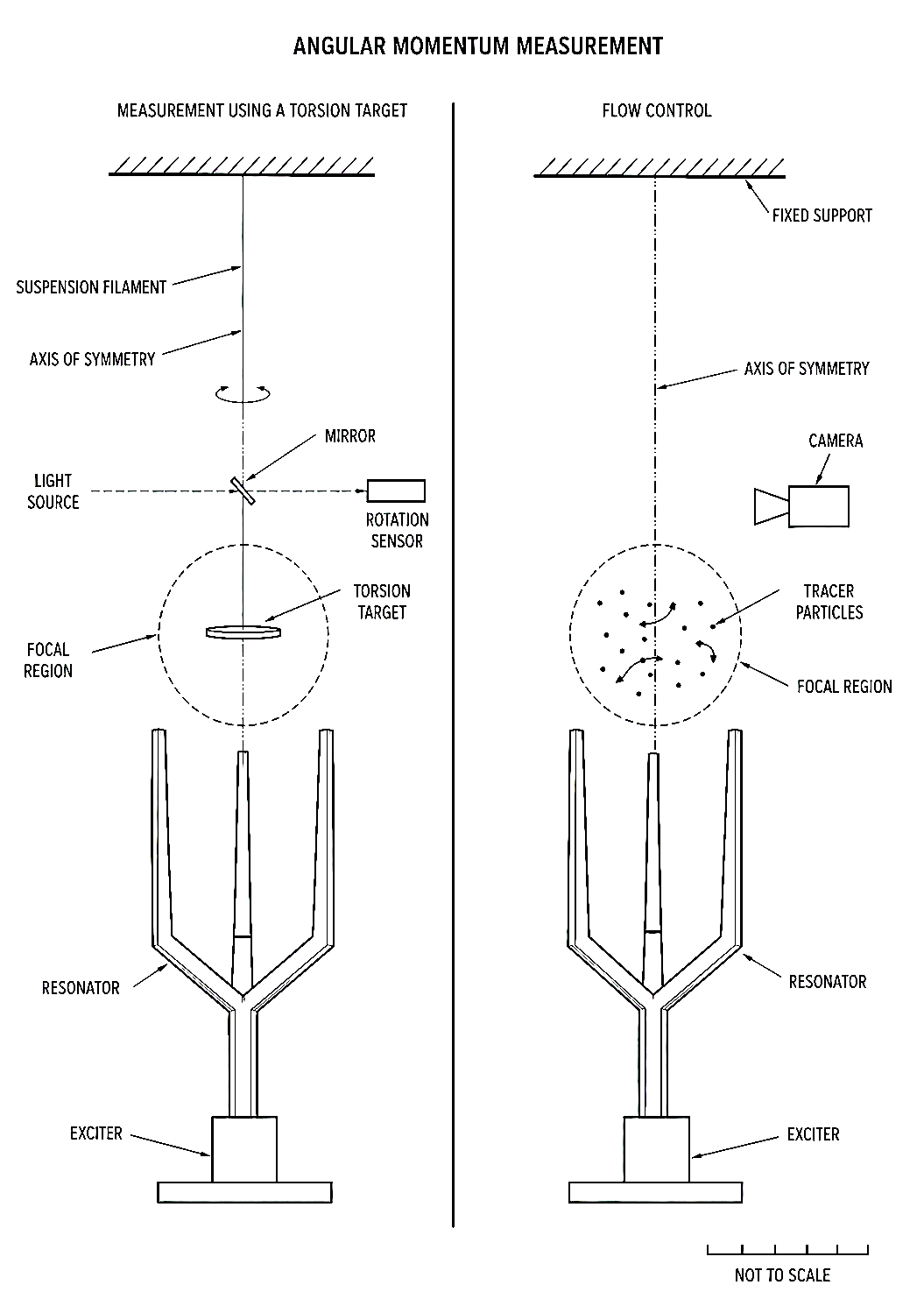
9.7 Scale and its implications
This subsection calibrates the preceding claims against the ratio of a characteristic resonator dimension to the acoustic wavelength.
At fundamental frequencies in the hundreds of hertz, the wavelength of sound in air is on the order of tens of centimeters to approximately one meter, while the characteristic dimension of the resonator is substantially smaller. In this frequency range, the resonator therefore operates in a regime where its size is small relative to the wavelength.
For subwavelength sources, generating a strongly structured and directionally stable far field becomes increasingly difficult. Higher spatial components of the field radiate less efficiently, and a substantial fraction of the structure may remain bound to the near field of the source. This is therefore not a sharp threshold of "present versus absent," but a gradual change in efficiency and spatial character as the ratio of source size to wavelength changes.
For a Triaural resonator, this means that at audible frequencies, rotating or phase-circulating structures anticipated under H-N1-01 and H-N1-06 must first be sought in the near field, where spatial structure may be more pronounced than in the far field. If a radiated vortex beam or orbital angular momentum carried into the far field is to be tested, the decisive parameter is the ratio of the characteristic resonator dimension D to the wavelength λ.
Accordingly, every measurement reports at least the dimensionless ratio
(D)/(λ),
or the equivalent wave parameter
kD=(2πD)/(λ),
where D is the selected characteristic dimension of the resonator and k is the acoustic wavenumber.
Interpretation of the results will distinguish the near field, transition region, and far field. The same geometric structure may exhibit different amplitude and phase organization in these regions, so conclusions from one region should not be transferred automatically to another.
The scale question is developed further in Chapter N1/09.12, which examines the transition to smaller resonators and higher operating frequencies.
9.8 State of the art: how acoustic vortices are generated today
To define the object of study precisely, it must be distinguished from the methods used in existing systems to generate acoustic vortices and other fields with azimuthal phase progression. For the purposes of this document, three working classes can be distinguished according to the origin of the spatial phase organization.
Class A - actively phased source
This class includes arrays of multiple transducers whose amplitude and phase are controlled electronically. Examples include phased arrays, holographic acoustic tweezers [25], systems with controllable topological charge [26], and the generation of structured surface acoustic waves using inverse control [27].
In this case, the azimuthal phase structure is imposed by the excitation signals. Changing the electronic phasing can therefore alter the properties of the resulting field without mechanically changing the array itself.
Class B - passive wave transformer
The second class consists of structures that spatially transform a wave produced by a separate source. These include spiral phase plates [28], metasurfaces and metamaterial apertures [29, 30], acoustic holograms [31], spiral diffraction gratings [32], and other passive elements designed to generate a desired phase profile.
This group can also include systems in which the radiating structure itself is resonant or supports guided mechanical waves, provided that the desired azimuthal phase structure is determined by a structural or excitation element that deliberately introduces it into the system. Examples include a resonator layer with azimuthally segmented sectors [34] or an elastic structure in which guided flexural waves generate a field carrying orbital angular momentum when radiating into a liquid [35].
Class C - intrinsic modal dynamics of the resonator
For the purposes of this document, working Class C denotes a case in which a spatially progressing phase structure would arise from the intrinsic modal dynamics of a finite resonator, without an electronically imposed azimuthal phase gradient and without a separate passive element intended to create it.
The primary subject of investigation is the possibility that a degenerate pair belonging to the nonsymmetric modal class of a three-pronged body may, under certain conditions, form a rotating superposition as described in Chapter N1/09.3. The existence of a degenerate pair alone does not guarantee such a state. Experiment must determine whether the required amplitude and phase relationship develops under a particular excitation method and whether the resulting spatial structure is measurable.
Within the literature corpus examined under protocol N1/02.5, no work was identified that unambiguously demonstrated the same case: a three-pronged monolithic resonator with the relevant rotational symmetry in which measurable azimuthal phase circulation arose from the resonator's intrinsic modal response without a deliberately imposed azimuthal phase gradient. This conclusion applies only to the scope of the literature search performed and is not a claim of absolute novelty.
What Class C must demonstrate experimentally
The decisive test is not the existence of an acoustic vortex as such; that phenomenon is already known [14]. Nor is it sufficient to demonstrate that a mechanically vibrating body can radiate a field carrying orbital angular momentum.
To classify the investigated resonator within working Class C, a link must be demonstrated between its intrinsic modal structure and the observed phase progression. The measurement must therefore determine:
- whether the resonator contains the predicted degenerate or nearly degenerate pair;
- whether the selected excitation method establishes a time-defined amplitude and phase relationship between its components;
- whether this mechanical state corresponds to a spatially progressing phase in the acoustic field;
- how the result changes under controlled symmetry breaking or a change in excitation method.
A particularly strong test is impulsive or in-phase excitation, in which no azimuthal phase gradient is deliberately imposed by the excitation system. If reproducible phase circulation is demonstrated even under these conditions, together with a link to the resonator's intrinsic modes, this constitutes a direct test of the mechanism defined for this working class.
Potential applications of acoustic fields carrying orbital angular momentum include, for example, contactless particle manipulation, imaging, and information transfer [36, 37]. In this document, these are presented only as technological context and do not constitute claims regarding the applicability of a specific Triaural resonator.
9.9 Dual-frequency excitation and difference-frequency dynamics
If the resonator is excited simultaneously at two nearby frequencies f_1 and f_2, their linear superposition produces an amplitude- and phase-modulated response with a characteristic time scale determined by the difference
Δf=∣f_2-f_1∣.
This difference frequency describes the rate of change of the envelope or of the relative phase between the two components. In a linear system, however, it does not by itself constitute a new, independent acoustic frequency component.
If each excitation frequency has a different spatial modal or phase structure, their superposition can create a field whose amplitude maxima, minima, or phase evolve over time on the time scale Δf. This evolution can be much slower than the carrier oscillations f_1 and f_2, while the spatial structure remains determined by the higher frequencies and the corresponding resonator modes.
This makes it possible to separate two time scales experimentally: fast mechanical and acoustic oscillation at f_1 and f_2, and the slower temporal evolution of their superposition at Δf. Such a regime may be useful for observing precession, pulsation, or periodic reorganization of the modal pattern, especially when two nearby natural frequencies or a split degenerate pair are excited.
Difference-frequency component produced by nonlinear mixing
True frequency mixing must be distinguished from linear beating. If the system contains sufficiently strong nonlinearity, new components may appear in the frequency spectrum, including a difference-frequency component:
f_DF=∣f_2-f_1∣.
Such a component is a distinct product of nonlinear interaction and must be demonstrated directly in the spectrum. Its existence cannot be inferred merely from the presence of two excitation frequencies.
For the Triaural resonator, two questions must therefore be distinguished: whether dual-frequency excitation produces a slowly evolving spatial superposition in the linear regime, and whether a measurable nonlinear component at the difference frequency also appears at higher amplitude. This is hypothesis H-N1-57.
9.10 Evidence to date
The following observations arose during device development and are not results of systematic measurements. They are included because they led directly to the hypotheses formulated in this document - and they are presented with all of their limitations.
They are therefore indications, not evidence, and in this text they carry the [O] register defined in Chapter N1/01.3. Their purpose is to show where the questions came from, not to answer them.
We intentionally include observations that may later prove to be artifacts. Omitting an observation because it was not confirmed would be worse than reporting it together with a clear statement of its weaknesses.
Overview of observations:
• Cymatics at a water surface - comparison of a two-pronged and a three-pronged tuning fork. Photographic and video record from July 11, 2025, with the prongs immersed in water. Resonator material: aluminum; water depth: 4 cm; vessel: plastic cylinder 7.5 cm high and 10 cm in diameter. No control measurement.
• Rotational motion of metal filings in a circular vessel positioned in the crown of the resonator. At certain excitation frequencies, directional motion of the filings along circular or approximately circular trajectories was repeatedly observed. Experimental conditions were not recorded systematically and repeatability was not quantified. The observation therefore does not identify the mechanism of motion and may involve multiple mechanical, acoustic, or flow-related influences.
• Deposition of dissolved mineral in a test tube containing Fatra mineral water placed in the focal region of the EMT. Photographically documented. The pattern gradually dissolved after opening and handling, suggesting a metastable structure. Frequency, exposure time, and exact water composition were not recorded; no control sample was used. The methodological implications are developed in Chapter N1/11.
• Filaments above the free ends of the prongs in a glass chamber filled with glycerol mist. After the flow stabilized, two to three filament-like structures were observed extending upward and slightly outward. The observation was not recorded; the frequency and power are unknown. Possible mechanisms are discussed in Chapter N1/10.10.
• Characteristically longer ring-down at the resonator's native frequency. During work with the EMT, a longer ring-down was repeatedly perceived subjectively at approximately 1045 Hz compared with other excitation frequencies. The observation was not quantified.
• Subjectively reported change in the taste and perceived density of water after exposure. The observation was neither quantified nor blinded. A proper verification method is described in Chapter N1/11.7.
• Kinematics of the free ends of a three-pronged resonator with rectangular prong cross-sections in slow-motion video. A frame-by-frame review shows predominantly symmetric inward and outward motion of all three prongs, corresponding to a "breathing" pattern. At the same time, individual time intervals show deviations from perfect symmetry: the projected displacement of one prong may temporarily decrease relative to the others, and a similar effect appears for different prongs at different times. The recording was made from an oblique angle and without spatial calibration, so the true three-dimensional trajectories or phase relationships between the prongs cannot be determined from it. The observation is compatible with a superposition of multiple modal components, but by itself does not distinguish between standing, rotating, and hybrid states. Systematic verification requires synchronous spatial measurement of the motion of each prong, for example using a sufficiently high-resolution high-speed camera or laser vibrometry.
• Change in the sound response after mechanical loading of one prong. In a freely vibrating three-pronged resonator, pronounced rapid amplitude modulation of the ring-down was observed subjectively. After one prong was mechanically loaded with a clamp, this modulation weakened markedly or disappeared and the ring-down was perceived as a more stable tone. The load simultaneously changes the mass, stiffness, damping, and boundary conditions of one prong, so the observation cannot be interpreted unambiguously as splitting of a degenerate pair. It nevertheless provides a useful basis for a controlled experiment involving deliberate symmetry breaking.
• Spatial minima and changes in the sound field around a continuously driven resonator in the EMT. As the measurement point or listener moved around the resonator, pronounced spatial differences in sound amplitude and character were repeatedly observed; in some positions, the apparent source location also changed. At certain locations, amplitude pulsation was audible during a continuous tone. The observation has not been systematically mapped or phase-measured, so it is not yet possible to distinguish between interference minima, modal superposition, motion-related effects, or a combination of these.
Working scenarios of modal behavior
Preliminary observations of prong kinematics do not allow a single mode of vibration to be assigned to the three-pronged resonator. Three working scenarios are therefore distinguished for systematic measurement:
Scenario A - predominantly symmetric state.
The resonator motion is composed primarily of a symmetric modal component. The three prongs deflect approximately simultaneously inward and outward, with no stable directional phase progression demonstrated between the prongs.
Scenario B - predominantly rotating nonsymmetric state.
The motion contains a nonsymmetric modal component with a stable directional progression of phase or displacement maxima between the prongs. The spatial pattern therefore progresses around the resonator's central axis.
Scenario C - hybrid state.
Measurable symmetric and nonsymmetric modal components are present simultaneously. Their relative contributions may differ: the symmetric "breathing" response may dominate with an added nonsymmetric component, or the nonsymmetric response may dominate with a measurable symmetric contribution. The relative contributions of the components may also change during ring-down.
These scenarios do not represent three mutually exclusive properties of the resonator. Depending on excitation method, frequency, mounting, geometric symmetry, and the course of ring-down, the same specimen may move between different proportions of the individual modal components. Distinguishing them therefore requires time-synchronized measurement of the amplitude and phase of motion of each prong.
Scenarios A-C are a working classification and do not exhaust all possible forms of modal behavior. Experiment may reveal responses that cannot be assigned unambiguously to this classification; in that case, the classification will be extended according to the measured data.
H-N1-64 - Under selected excitation conditions, vibration of a three-pronged resonator may simultaneously contain measurable symmetric and nonsymmetric modal components.
- Confirmation: synchronized measurement demonstrates, within the same time interval, contributions from both the symmetric and nonsymmetric modal components above a predefined threshold of measurement uncertainty.
- Falsification: within the preregistered set of tested conditions, the motion can be described consistently without simultaneous presence of both components above the predefined measurement-uncertainty threshold.
9.11 Connections to other fields
Threefold symmetry, modal degeneracy, and rotationally organized fields also appear in other areas of physics. The following examples are presented as mathematical or geometric parallels. They do not imply that the individual systems share the same physical mechanism.
Geometric frustration in magnetism
If three magnetic moments are arranged in a triangle and their mutual interactions favor antiparallel alignment, all three pairwise interactions cannot be satisfied simultaneously. In a simple symmetric case, a 120° arrangement may emerge as a compromise state.
The parallel with the Triaural resonator is that threefold symmetry constrains the set of permitted collective states of the system. The physical mechanism is different, however: magnetic frustration involves energetic competition among interactions, whereas the resonator involves the modal structure of an elastic body.
Toroidal moments in electrodynamics
In electrodynamics, toroidal moments are described alongside electric and magnetic multipoles and arise from particular spatial arrangements of currents. Such configurations can have pronounced internal field structure while exhibiting radiation properties different from those of simple electric or magnetic dipoles.
The parallel with the Triaural resonator is exclusively structural: in both cases, the spatial organization of multiple contributions can produce a resulting field whose properties depend on their common geometry and phase relationships. The document does not infer from this similarity the existence of a toroidal electromagnetic moment in the resonator.
Vortical structures in hydrodynamics
Hydrodynamic systems can form circulating velocity fields and vortex structures characterized by circulation or vorticity. The acoustic phase singularity described in Chapter N1/09.5 is a different phenomenon: it is a singularity of the phase of a complex wave field, not automatically a vortex of the time-averaged velocity of the medium.
The parallel lies in the existence of organized circulation around a particular region or axis. Experimentally, however, these phenomena must be distinguished because acoustic phase circulation and hydrodynamic flow can exist separately or simultaneously.
Common denominator
The common denominator among these examples is the role of symmetry and collective organization in generating properties of the overall system. These are parallels at the level of mathematics, geometry, or field organization; the individual physical mechanisms remain distinct. Their inclusion therefore places the investigated problem in a broader physical context rather than serving as evidence for the hypotheses formulated in this document.
9.12 Scale branch: transition to ultrasound
The ratio of a characteristic resonator dimension to wavelength strongly affects how its spatial structure is transferred into the surrounding acoustic field. At audible frequencies, the investigated resonator is generally a subwavelength source, and a substantial part of the complex spatial structure may therefore appear primarily in the near field, as discussed in Chapter N1/09.7.
As frequency increases, wavelength decreases and the ratio D/λ increases for the same or a reduced geometric form. This changes the radiation conditions for higher spatial components and makes it possible to examine whether the resonator's modal structure produces measurable azimuthal phase organization beyond the immediate near field.
For example, at 440 Hz the wavelength of sound in air is approximately 78 cm, whereas at 40 kHz it is approximately 8.6 mm. A resonator with a characteristic dimension on the order of tens of millimeters therefore operates at an ultrasonic frequency in a very different dimension-to-wavelength regime than a geometrically similar resonator in the audible range.
The transition to ultrasound therefore does not change the fundamental research question. It allows the same relationship among geometry, modal structure, and acoustic field to be investigated in a different scale regime.
Direct mapping of phase structure
Phase circulation can be mapped experimentally in both the audible and ultrasonic ranges. The ultrasonic scale, however, allows more compact setups and source-size-to-wavelength ratios comparable to those of many systems used in existing acoustic-vortex research.
Spatial scanning records the complex acoustic pressure, including both amplitude and phase. A candidate phase singularity is identified by the combination of a local amplitude minimum and a nonzero integer phase winding along a closed path around the relevant point or axis.
An amplitude minimum alone is therefore insufficient. Visual observation of rotating particle motion alone is likewise insufficient. The decisive evidence is the combination of a spatial amplitude-and-phase map with an independent measurement of the mechanical state of the resonator.
What is measured
- amplitude and phase map of the acoustic field in planes perpendicular to the Triaural axis;
- location of any phase singularities and their evolution with distance from the resonator;
- topological charge calculated from phase winding along a closed contour;
- amplitude and phase of the mechanical motion of the individual prongs;
- torque transfer to the torsion target according to Chapter N1/09.6;
- any particle motion or rotation while simultaneously controlling for acoustic streaming;
- dependence of these quantities on excitation method, frequency, geometric deviation, and the ratio D/λ.
Laser vibrometry provides an important independent control here: if the acoustic phase structure is to be attributed to a degenerate pair, the amplitude and phase behavior of the resonator itself must be known simultaneously.
Hypotheses of the scale branch
Related hypothesis H-N1-06: At a sufficiently large ratio of characteristic resonator dimension to wavelength, excitation of the degenerate pair in quadrature will produce an acoustic field with measurable nonzero orbital angular momentum.
H-N1-60: Under excitation without a deliberately imposed azimuthal phase gradient, a three-pronged resonator may produce reproducible phase circulation in the acoustic field that is linked to its intrinsic modal dynamics.
- Confirmation: under excitation without a deliberately imposed azimuthal phase gradient, nonzero phase winding is demonstrated reproducibly together with a temporal relationship to the measured modal response of the resonator.
- Falsification: under preregistered conditions, phase circulation appears only when an azimuthal phase gradient is imposed by the excitation method or by a separate shaping element, or no measurable circulation is demonstrated at all.
H-N1-61: The fundamental rotating state associated with the nonsymmetric degenerate pair of a three-pronged resonator will produce a phase singularity with topological charge ∣l∣=1, with the sign of l reversing when the direction of phase circulation is reversed.
- Confirmation: the phase map shows a total phase change of approximately +2π or -2π around a closed path enclosing the singularity, and the sign of the charge reverses under controlled reversal of the circulation direction.
- Falsification: the fundamental reproducible state shows a different topological-charge magnitude, zero phase winding, or no reversal of sign when the direction of circulation is reversed.
H-N1-62: Controlled breaking of threefold symmetry will systematically change the position, stability, or topological structure of the phase singularity associated with the rotating state.
- Confirmation: as the defined deviation from C3 symmetry increases, at least one predefined characteristic of the singularity - its position, stability, number, topological charge, or existence - changes reproducibly in correlation with the change in modal splitting.
- Falsification: over the investigated range of geometric deviation, these characteristics do not change beyond measurement uncertainty and show no systematic relationship to modal splitting.
H-N1-63: In geometrically similar three-pronged resonators, the character of the modal and acoustic rotational response will be preserved across different scales when the relevant dimensionless system parameters, including the ratio of characteristic dimension to wavelength, are comparable.
- Confirmation: after normalization of spatial coordinates and relevant frequency and amplitude quantities, geometrically similar resonators at different scales exhibit the same or statistically comparable class of modal and phase structure.
- Falsification: at comparable relevant dimensionless parameters, reproducible differences arise between scales that cannot be explained by measurement uncertainty or known material or loss mechanisms.
Hypothesis H-N1-60 is a direct test of working Class C defined in Chapter N1/09.8. Its decisive feature is excitation without a deliberately imposed azimuthal phase gradient together with demonstration of a link between any phase circulation in the acoustic field and the resonator's intrinsic modal dynamics. This experimentally distinguishes it from working Classes A and B, in which the desired spatial phase profile is intentionally created by source control or a shaping element.
Implications for the program
The ultrasound branch anticipates specimens with characteristic dimensions on the order of units to tens of millimeters. Their manufacture therefore requires precise control of geometry, cross-sections, and surface condition. The suitability of a particular manufacturing technology - machining, micromachining, additive manufacturing, or casting - will be assessed according to the required tolerance and material.
When scale is changed, natural frequencies, quality factor, damping, and modal splitting are measured independently. Their evolution cannot be inferred from geometric scaling alone because the relative contributions of material, surface, thermoelastic, and fluid losses may change.
Safety requirements for airborne ultrasound are evaluated separately under Chapter N1/18 and the applicable exposure limits.
Conclusion:
The ultrasound branch therefore represents a test of geometric and modal similarity, not an assumption that such similarity automatically holds. If the same type of modal and phase behavior appears across different scales after accounting for the relevant dimensionless parameters, this would support the hypothesis that the observed mechanism is a property of the resonator's geometric-modal organization rather than a peculiarity of one specific frequency or size.
CYMATICS AND THE ACOUSTIC HOLOGRAM - A FIELD THAT CAN BE SEEN AND HEARD
Sound is invisible, but it can be projected into matter in a way that makes it visible. This chapter turns a compelling image into a measurement method.
Left side: Right side:
Conventional two-pronged tuning fork Triaural three-pronged tuning fork
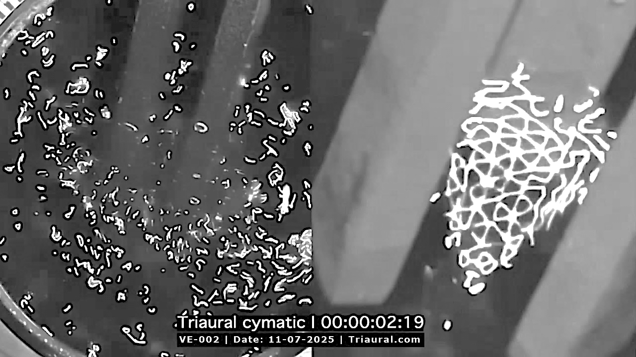
Source: triaural.com / 1.) Photo report ZIP, 2.) Cymatics video report, 3.) Cymatics comparison video report 2 vs 3 / download:
10.1 From image to method
Cymatics is usually presented as an image. Fine powder on a vibrating plate or the surface of a liquid forms a pattern, and a photograph of that pattern can be persuasive even without words [40, 41].
For measurement purposes, the image must be converted into a quantity. This requires three things: the pattern must be produced under recorded conditions, captured with a calibrated setup, and evaluated computationally. Only then can patterns from two different sources be compared and their differences described.
This chapter therefore treats cymatics as a measurement method. It addresses what the pattern represents, how its shape is quantified, which controls are required, and where the limits lie on what can be inferred from it.
10.2 What the pattern represents
A pattern on a plate or liquid surface represents the spatial distribution of nodes and antinodes within a thin layer. For granular material with sufficiently massive particles, the particles accumulate where displacement is smallest and leave regions where it is greatest. The resulting pattern therefore represents a spatially selective response of the medium to the local distribution of vibration or the acoustic field. In a classical Chladni setup, its geometry is closely related to the nodes and antinodes of the plate's natural modes; for an inserted medium or a free liquid surface, however, the dynamics of the medium itself and its boundary conditions must also be considered.
For very fine and lightweight powder, the opposite can occur. The particles are carried by airflow above the plate and accumulate instead in regions of strongest vibration; Chladni himself observed this with fragments of bow hair [42]. The type and grain size of the granular material therefore determine whether the pattern maps nodes or antinodes, and they must remain unchanged within a comparative series.
A free liquid surface introduces an additional mechanism. Under vertical excitation above a threshold amplitude, the liquid surface can form its own regular patterns - stripes, squares, or hexagons - whose symmetry arises from the hydrodynamics of the liquid. This is the Faraday instability, discussed in detail in Chapter N1/11.
This establishes a condition for interpretation. The observed pattern may contain simultaneous contributions from the driving field and from the liquid's own hydrodynamic response. Their separation is addressed by the rotation test in Chapter N1/11.4.
For a radial resonator, this determines the order of methods. A plate in a classical Chladni setup vibrates in its own modes, and the pattern maps those modes. A solid object inserted into the field of a three-pronged resonator also has natural modes of its own, so the resulting pattern would map those modes rather than the driving field.
The primary method is therefore a free liquid surface, where no discrete elastic mode of an inserted plate is introduced; the vessel geometry, liquid depth, and hydrodynamic boundary conditions must still be controlled. A secondary method uses a plate or tensioned membrane placed in the field, always with explicit consideration of the inserted body's own modes and with the rotation test defined in Chapter N1/11.4. A third branch uses a granular layer into which the prong tips are immersed. Unlike a liquid surface, the resulting pattern remains after excitation stops and can therefore be imaged without a stroboscope and after a delay.
10.3 Pattern quantification
The pattern shape is converted into numerical values using two independent procedures that measure different properties.
The first procedure analyzes the boundary of the region in which material has accumulated. The distance from the boundary to the centroid is expressed as a function of angle and decomposed into harmonic components. The amplitude of the component of order n indicates the degree of n-fold symmetry of the boundary and is compared with the noise level represented by the remaining orders.
The second procedure analyzes the internal texture. A two-dimensional Fourier transform converts spatial repetition in the image into an angular power spectrum. A sixfold lattice appears as a sixth-order component. In an ideally symmetric pattern, dominant harmonic components corresponding to its rotational symmetry are expected; in real images, additional orders may appear because of asymmetry, noise, illumination, or imperfect segmentation.
The analysis is repeated at several levels of image smoothing. Large-scale structure may not appear at a fine scale and vice versa; examination across scales is therefore part of the procedure.
A summary quantity derived from these decompositions is referred to in this document as the triaurality index. Its exact definition will be established after the first measurement series, once the range of values observed in real samples is known.
In this document, the triaurality index is introduced as a provisional summary metric. Its final definition, normalization, and reference ranges will be established before the main comparative series using an independent calibration dataset and will remain fixed during subsequent evaluation.
The index is based on two values. The first is the ratio of the amplitude of the third-order component to the sum of the amplitudes of all orders in the boundary decomposition. The second is the same ratio in the angular power spectrum obtained from the two-dimensional Fourier transform. Both are dimensionless and, by construction, range from zero to one.
The range over which the index is informative will be determined from the variability of repeated measurements on the same specimen. If the difference between two specimens is smaller than this variability, the index does not distinguish them; the result is reported as indistinguishable, not identical.
After the first series, the definition will be recorded together with the date and the data from which it was derived, and it will not be changed thereafter. Recalculation of earlier measurements using a new definition is permitted only if both values are reported.
10.4 Controls and artifacts
Every series includes three controls that are performed each time.
An unexcited control sample held for the same duration and at the same temperature shows how much of the pattern arises from evaporation and settling. The rotation test in Chapter N1/11.4 distinguishes whether the pattern is linked to the source or to the vessel. A control source with different geometry is measured at the same frequency, comparable excitation amplitude or acoustic pressure at a defined reference point, the same position, and the same exposure time. Differences between the patterns can then be tested as a function of source geometry.
The type, grain size, and mass of the granular material are recorded and kept constant within a comparative series. Imaging is performed perpendicular to the pattern plane, with a scale marker and constant illumination. Perspective distortion is corrected before analysis; a circular region viewed at an angle appears elliptical and produces a dominant second-order component in the harmonic decomposition.
Evaluation is blinded. Images from exposed and control samples are coded and analyzed together without knowledge of their assignment.
10.5 Laser mapping of the nodal network
Reflection of a narrow laser beam from a liquid surface or reflective surface converts local surface slope into displacement of the reflected spot. The method can therefore detect small changes in slope that may not be apparent in the cymatic pattern itself.
By scanning over a defined grid, a map of the local surface response can be constructed. For periodic vibration, acquisition is synchronized with excitation or evaluated with time resolution so that the oscillatory component can be separated from static slope.
Spatial resolution is determined by the combination of scan step, laser spot diameter, optical-path geometry, sensor resolution, and signal-to-noise ratio. The method therefore provides an independent complement to image-based analysis of particles or the liquid surface.
10.6 Position of the amplitude minimum
A surface pattern represents a two-dimensional section through the response of the medium, whereas the region under study above the central node is three-dimensional. A single pattern therefore cannot determine the height or position of a local minimum in the measured quantity.
The spatial position of the minimum is determined by measurements in multiple planes while the resonator geometry, position, and excitation method remain unchanged. The measurement plane or sensor is moved along the Triaural axis, and at each position the amplitude response - and, where the method permits, the phase response - is recorded.
If series with different liquid levels or different immersion depths of the prongs are used, they are treated as separate experimental configurations because changing immersion alters the fluid loading of the resonator and the boundary conditions of the system. Without additional controls, they cannot be interpreted simply as sections through the same unchanged field.
The result is the spatial dependence of the position and depth of the amplitude minimum along the axis; its relationship to the central node and the defined focal region is then tested experimentally.
10.7 Relationship to quality factor
Under impulsive excitation, the quality factor may affect the time for which the medium experiences sufficient amplitude to form an observable pattern. With rapid ring-down, the resulting pattern may therefore be less pronounced or more variable, while the specific response also depends on the dynamics of the medium.
The measurement therefore includes simultaneous recording of the ring-down and the time evolution of the pattern. With controlled continuous excitation through FORKER, the amplitude can be maintained at a defined level, substantially reducing the influence of different ring-down durations between specimens. This is one reason comparative series are performed at the appropriate controlled level of the complexity ladder.
10.8 Blinded classification test
The question of whether a pattern carries a signature of source geometry can be converted into a task with an unambiguous criterion.
A classifier is given images of patterns produced by two-pronged, three-pronged, and four-pronged sources at the same frequency and amplitude and assigns each image to a source topology. Training and test sets are separated, coding is blinded, and perspective is corrected.
The criterion is classification accuracy above chance at a predefined level of statistical significance on an independent test set. If the classifier reproducibly performs above chance, the patterns contain information that allows the source topology to be distinguished. If it does not reach this level, no such distinguishable information has been demonstrated in that experiment with the method used.
A negative result does not by itself demonstrate complete independence of the pattern from source geometry; it establishes an upper bound on distinguishability for the given data quality and analytical procedure.
The task remains within acoustics and image processing. The result concerns the distinguishability of the patterns and does not determine the mechanism by which they arise. This is hypothesis H-N1-54.
The split between training and test data is performed at the level of independent experimental runs or specimens, not by randomly dividing individual frames from the same recording.
The task remains within acoustics and image processing. The result concerns pattern distinguishability and makes no claim about the mechanism by which the patterns arise.
10.9 Volumetric visualization
Cymatics provides a two-dimensional response of a medium in a single plane. An aerosol in a closed chamber makes it possible to observe the spatial transport and concentration of tracer particles throughout a volume, thereby examining volumetric flow or other mechanisms that may not appear in a planar pattern.
Initial observation: after the EMT glass chamber was filled with glycerol mist and the flow was allowed to settle, two to three thin aerosol-free filaments formed just above the free ends of the prongs, extending upward and slightly outward. The observation was made under provisional conditions, could not be recorded because of demanding lighting conditions, and the excitation frequency was unknown; its status is given in Chapter N1/09.10.
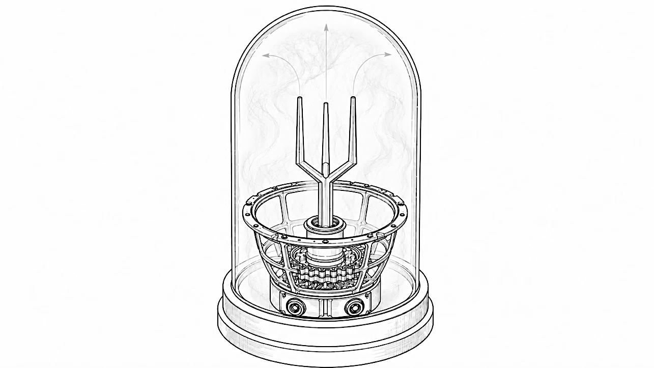
10.10 Candidate mechanisms
Possible explanations are stated before measurement so that selection among them follows from the result rather than the other way around.
The first candidate is acoustic streaming generated near the vibrating prong tips. Its direction and structure depend on amplitude, geometry, medium viscosity, and boundary conditions. If the filaments are caused primarily by local flow near individual prongs, their position should correlate systematically with the position and motion of the tips.
The second candidate is acoustically induced redistribution of droplets in a standing or spatially structured field. Local differences in acoustic pressure and particle velocity can alter aerosol concentration and create regions of higher or lower particle density.
The third candidate is local changes in droplet size or concentration caused by thermal or pressure-dependent processes.
The fourth is thermal convection from the base, coil, or heated resonator. This mechanism is unrelated to sound and is a major potential source of error.
10.11 Frequency discrimination test
One measurable dependence can help distinguish among these mechanisms. If the characteristic spacing of the filaments is directly linked to the acoustic wavelength, an approximately inverse dependence on frequency is expected when all other conditions remain unchanged. In the ideal case, doubling the frequency would produce approximately half the characteristic spacing.
A deviation from this relationship would not automatically rule out an acoustic mechanism, because the result may also be influenced by the resonator's modal structure, chamber geometry, and transitions between different flow regimes.
Thermal convection does not scale with acoustic frequency. Tip-driven flow may change in intensity while leaving the characteristic spacing unchanged.
The characteristic filament spacing is therefore measured over a series of frequencies and tested for an approximately inverse dependence on frequency over the range in which the other experimental conditions remain comparable. Deviations from this behavior are evaluated together with changes in modal regime, amplitude, and flow geometry. This is hypothesis H-N1-41.
10.12 Control measurements for volumetric visualization
An aerosol without excitation over the same duration shows what arises from buoyancy and heat. A rotation test, in which the resonator is rotated relative to the chamber, distinguishes structures tied to the prongs from those tied to the vessel. Temperature is recorded inside the chamber and on the surface of the base throughout the experiment. Illumination of the base is turned off as a separate control.
The series is repeated with the same aerosol and flow conditions using a resonator that is mechanically present but not excited, separating the effect of the resonator geometry on natural convection.
Before each measurement, the time required for the aerosol to settle after filling the chamber is recorded, and the experiment begins only after a defined quiescent state has been reached.
10.13 Seeding medium and imaging
Glycerol aerosol is a suitable candidate tracer medium because, with an appropriate droplet-size distribution, its droplets can remain suspended for relatively long periods and offer good optical visibility. The ability to track flow nevertheless depends on droplet size, particle inertia, and the characteristic time scale of the flow; these parameters are therefore controlled or estimated in quantitative measurements. Water aerosol may be less stable over time because of faster evaporation and changes in droplet size, so its suitability is evaluated separately.
The missing element in the previous trial was illumination. Under diffuse light, the fine structure is below the resolving capability of a conventional camera.
The solution is a laser light sheet. A thin plane of light cuts through the volume, the camera views it from a perpendicular direction, and the background remains dark, producing a sharp section rather than a hazy volume. The same type of setup is also used for laser mapping as described in Chapter 10.5.
10.14 Quantitative evaluation
Imaging the illuminated plane in pairs of frames separated by a short interval allows the velocity field to be calculated using image-correlation methods. With a sufficiently dense tracer-particle field, successive image pairs can be evaluated using PIV (Particle Image Velocimetry), which yields a two-dimensional velocity field in the illuminated plane. With a sparser set of well-resolved particles, PTV (Particle Tracking Velocimetry) can be used to follow individual trajectories. Outputs include local velocities, flow directions, recirculation regions, and possible vortex cores.
H-N1-42: In a regime dominated by acoustic streaming, the characteristic time-averaged flow velocity increases approximately with the square of the acoustic or mechanical excitation amplitude over the preregistered range.
When PIV/PTV is used, volumetric visualization is primarily a method for observing material transport in the medium, corresponding to Path B in Chapter N1/09.5. A phase singularity of the complex pressure field is not determined directly by this measurement and must be mapped separately.
Preliminary observation of particle transport
A separate preliminary observation involved the motion of metal filings in a round vessel mounted in the crown region of the resonator. At some excitation frequencies, video recordings showed directional particle motion with a pronounced circumferential component. The frequencies and other experimental conditions were not recorded systematically, and repeatability was not quantified; the observation therefore has status [O] according to Chapter N1/09.10.
The recording by itself does not determine the cause of the motion. Candidate mechanisms include mechanical transmission of vibration into the vessel and particle layer, medium motion caused by acoustic streaming, asymmetric excitation of the setup, vessel geometry, or a combination of these factors. The observed circumferential transport therefore cannot be interpreted as evidence of phase circulation or transfer of orbital angular momentum.
In a repeat experiment, individual particle motion will be recorded from above using calibrated geometry and evaluated by PTV or trajectory-based image analysis. At the same time, the motion of the vessel and base will be recorded by vibrometry, and the amplitude and phase structure of the acoustic field will be mapped independently. This arrangement will make it possible to test whether the observed transport is associated with the support geometry, support motion, medium flow, or another component of the experiment. The direction of circumferential motion and its stability across repetitions will be recorded separately. If the direction of the imposed phase progression can be reversed in a controlled manner, the experiment will also test whether the direction of particle transport reproducibly reverses with it.
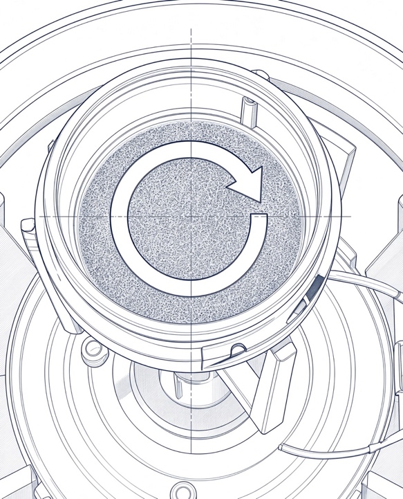
Video recording: Preliminary observation of rotation of iron filings in a dish: https://triaural.com/MULTIMEDIA/TRIAURAL_SAWDUST_ROTATION.mp4
10.15 Chamber scaling
In a small chamber, the walls may strongly influence the developing flow before its natural spatial structure can emerge. Chamber volume and shape, together with resonator position, are therefore varied systematically to determine whether the flow forms open streamlines, local recirculation regions, or a spatially closed recirculation cell. Hypothesis H-N1-43 tests whether closed recirculation emerges when the chamber volume is sufficiently large.
10.16 Acoustic hologram - a field that can be heard
The preceding sections address the field within the focal region and its immediate surroundings. During work with a continuously excited resonator, pronounced spatial differences in perceived loudness and sound character have repeatedly been noted subjectively even several meters from the source. Their physical structure has not yet been mapped systematically.
The question that unifies the following section is whether the spatial nodes are sections through the same structure visualized at the surface by cymatics - in other words, whether cymatics reveals planar sections through a volumetric structure. This is formally listed as open question Q-N1-07 in Chapter N1/22.3.
With the resonator sounding, listening can reveal points in space where the sound has a different loudness and timbre from points only a few centimeters away. The transition between them is distinct, and at an unchanged frequency their positions remain stable. This is an observation in register [O].
The term acoustic hologram is used in this document as a working name for a spatially organized distribution of amplitude and phase in the acoustic field. It does not refer to holography in the optical sense or to a passive holographic element of the type discussed in Chapter N1/09.8.
10.17 What acoustics says about this structure
For a simple standing wave, adjacent nodal surfaces occur at a spacing of approximately λ/2. In a more complex three-dimensional interference field, however, the spacing, shape, and orientation of amplitude minima depend on source geometry, phase relationships, propagation directions, and reflections from the environment.
The frequency dependence of the characteristic dimensions of the structure is therefore an important test, but it cannot be assumed in advance that all adjacent minima will be separated by exactly λ/2.
If a characteristic spatial dimension of the measured structure is directly linked to the acoustic wavelength, it is expected to change systematically with frequency. The specific relationship, however, depends on source geometry, phase relationships, and the presence of reflections; a simple scaling law is therefore tested as a special case rather than assumed as a general condition of an interference field.λ/2
Spatial amplitude minima also arise in enclosed rooms with conventional sources because of interference between direct and reflected sound. The mere existence of minima or a layered structure therefore does not demonstrate a special property of Triaural geometry. The decisive comparison concerns their amplitude and phase organization, how they transform when the source is rotated, and how they behave when the room or frequency is changed.
10.18 Layered structure
According to preliminary listening observations, regions of pronounced change in amplitude or sound character do not appear to form a single isolated surface but may occur in multiple spatial layers at increasing distance from the source. This pattern has not yet been mapped objectively, so the term “layered structure” remains provisional. As a visual analogy, the working concept can be compared to a set of separated shells around the source - like spaced layers of an onion; their actual shape, continuity, and regularity must be determined by measurement.
Measurement therefore cannot be limited to a single plane or a single spherical surface. Sampling is required across multiple layers at defined intervals to capture how the structure evolves with distance.
The quantities of interest are layer spacing, depth of minima, shape of nodal surfaces, and whether - and how - their orientation changes with distance, time, or frequency.
10.19 Measurement setup
The spatial structure is captured using a microphone array with synchronous recording of all channels. Synchronization is essential because phase, not only level, is recorded.
Scanning proceeds layer by layer. The array is placed at a selected distance, the entire surface is recorded, and it is then moved to the next layer. Layer spacing is chosen as a fraction of the wavelength so that the structure is not undersampled.
The measurement range is designed to extend from the immediate vicinity of the resonator to several meters away in order to capture the evolution of the field from the near region toward a region in which more distant radiation can be evaluated. The exact boundaries between near, transition, and far field are determined for the specific frequency and source dimensions.
A synchronized microphone array provides both amplitude and relative phase at each point and is therefore suitable for distinguishing true spatial minima from variations caused only by local level changes or room reflections.
Room conditions are recorded, including dimensions, reverberation time, and source position relative to the walls. Without these data, the source contribution cannot be separated from the room contribution.
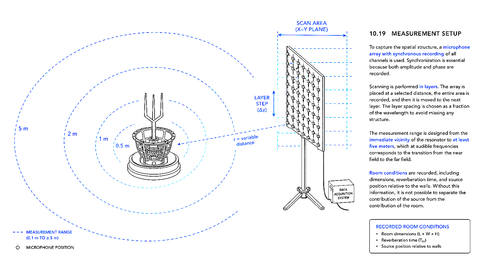
10.20 Controls
Separating the source contribution from the room contribution requires four controls.
- The same measurement is performed with a conventional source at the same frequency and level. The difference between the maps is the quantity of interest.
- Rotation of the resonator about its axis. Rotating the resonator about its axis tests which part of the map transforms with the source and which remains tied to the room. When both contributions are present, the resulting map may change through their combined effect.
- Changing the source position within the room. Nodes tied to the room will shift differently from nodes tied to the source.
- Changing the frequency and testing whether layer spacing changes approximately inversely with frequency.
Measurements are also repeated in a space with a different reverberation time, or, where feasible, outdoors where reflections are substantially reduced.
10.21 Perception of source location
At some positions, observations suggest that the sound appears to originate from a different location in the room, or in some cases from inside the listener's head. This is an observation in register [O]. Sound localization is based on comparison of the signals at the two ears, including differences in arrival time and level. One working possibility is that regions of low amplitude or steep spatial phase variation alter binaural localization cues, particularly interaural time and level differences. This may reduce externalization stability or shift the perceived source direction. Such effects are known in psychoacoustics and can be measured. The procedure compares a map of positions at which the phenomenon occurs with the measured field map and tests whether the phenomenon spatially coincides with amplitude minima or strong phase gradients. This interpretation is hypothetical and must be tested by comparing psychoacoustic mapping with the objective amplitude and phase map of the field.
10.22 Transmission through structures
According to preliminary observations, the sound of the resonator can be heard through walls and ceilings more strongly than might be expected from its apparent loudness. This is an observation in register [O], and two explanations must be separated.
The first is the transmission loss of the structure, which generally decreases toward lower frequencies. Airborne sound insulation in building structures is frequency-dependent, and attenuation at low frequencies can be substantially lower than at higher frequencies. The exact behavior depends on the composition and mechanical properties of the structure.
The second is structure-borne transmission. If the resonator stands on a support mechanically coupled to the building, part of the energy travels through the structure rather than through air, where attenuation can be much lower.
The two paths are separated by a simple comparison: the resonator is first placed on an isolating pad and then directly on the structure, while sound level is measured in an adjacent space. The difference between the two configurations provides an estimate of the contribution of mechanical coupling to the structure, not a direct absolute measure of the fraction carried by structure-borne transmission.
10.23 Independence from the monolith
Preliminary observations suggest that a spatially structured field may also be observed with multi-source arrangements without a monolithic resonator, for example with the AURISONIC configuration described in Chapter N1/12.6. Whether these fields are equivalent or different must be determined by measurement.
This branch is therefore independent of the L2/L3 result in the sense that the existence and geometry of a spatial interference structure remain measurable even if no specific contribution of the monolithic resonator is confirmed.
The related open questions are Q-N1-04 and Q-N1-05 in Chapter N1/22.3.
WATER AND LIQUID MEDIA
Water is one of the principal media in which responses to acoustic exposure are investigated - and also an environment in which an incorrect conclusion can be reached very easily. This chapter therefore pairs every observation with a corresponding control.
11.1 Why water
Water is one of the principal liquid media examined in this document. It makes it possible to observe, within the same system, the mechanical response of the surface, transport of dissolved or suspended substances, thermal changes, and other physical and chemical quantities using established measurement methods.
At the same time, water is an important reference medium for subsequent experiments involving biological systems, in which it constitutes a substantial part of the environment under study. This connection alone, however, does not justify transferring results obtained in water to a biological system.
Liquid samples are also sensitive to temperature, evaporation, dissolved gases, contamination, vessel geometry, and handling. When changes are small, observer expectation may also influence interpretation. For this reason, the chapter assigns control conditions and a measurement method to each quantity being monitored.
11.2 Initial observation and its status
A test tube containing mineral water was placed in the focal region of the EMT. After exposure, dissolved material became concentrated within a bounded zone on the surface instead of remaining evenly distributed.
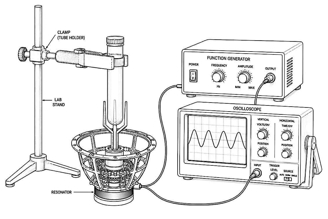
The observation was made under provisional conditions, without a control sample, calibrated imaging, or repetition. It is not presented as a result and does not serve as evidence for any claim.
When the vessel was opened and subsequently handled, the pattern gradually broke apart. The observation therefore does not establish whether it represented a metastable structure, a change induced by movement of the sample, disturbance of the surface, altered evaporation, or another mechanism. The practical consequence is nevertheless clear: the original state of the sample was not preserved during handling.
The repeat measurement is therefore performed in situ through a closed vessel, with a fixed camera position and no contact with the sample during either exposure or subsequent imaging.
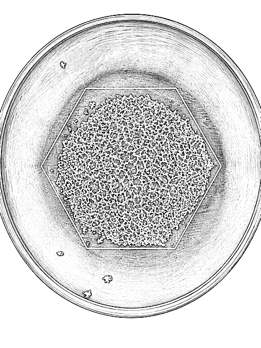
The question opened by this chapter is deliberately stated without assumption: does the deposition pattern exhibit measurable symmetry, and if so, what kind?
11.3 Faraday wave
Under periodic vertical excitation above a threshold amplitude, a liquid surface can enter a parametrically excited regime and form regular surface patterns. This phenomenon, historically associated with Faraday's experiment, is a standard subject of hydrodynamic-instability research [42].
The character of the pattern and the threshold for its formation depend, among other factors, on excitation frequency and amplitude, liquid depth, viscosity, density, surface tension, and vessel geometry. In the classical Faraday regime, the surface response may occur subharmonically relative to the driving frequency; the frequency relationship between excitation and response is therefore one of the measured quantities.
In a controlled experiment, excitation frequency and amplitude are set, while liquid depth, temperature, and physical properties are either defined or measured.
A separate measurement output is the threshold amplitude and a pattern map in frequency-amplitude space. Such a map can be compared with the literature and serves as a control for whether the setup behaves according to established physics.
The dominant frequency of the surface response is recorded simultaneously so that harmonic, subharmonic, and other response regimes can be distinguished.
11.4 Rotation test
One of the principal discriminating experiments in this chapter is a change in the relative angular orientation of the resonator and the vessel while all other conditions remain unchanged. The resonator may be rotated, the vessel may be rotated, or both variants may be performed; what matters is that the change in their relative orientation is known.
Measurements are performed at several predefined angles, for example 0°, 30°, 60°, and 90°, and the order of orientations is randomized across repetitions. After perspective correction, the patterns are compared using the same harmonic and image-analysis procedures described in Chapter N1/10.3.
If a particular component of the pattern reproducibly rotates with the resonator, this supports an association with source orientation. If it remains fixed relative to the vessel or the laboratory coordinate system, this supports an influence from the vessel, meniscus, gravitational orientation, illumination, or another stationary factor.
Both contributions may be present simultaneously. The resulting pattern therefore need not rotate as a rigid body; individual harmonics or spatial components may respond differently. The rotation test is therefore evaluated as the dependence of individual pattern components on the relative angle between the source and the vessel.
If the original pattern does not reappear in repeated measurements above the variability of control runs, the original observation is considered not reproduced. Non-reproducibility by itself, however, does not identify which particular random or uncontrolled factor produced the initial pattern.
The test is one of the principal controls for hypothesis H-N1-30.
11.5 Deposition as a record of the field
If exposure produces a reproducible deposition pattern, it can be studied as a spatial record of processes occurring in the sample during exposure. Deposition by itself, however, does not establish whether its geometry arose from the acoustic field, liquid hydrodynamics, evaporation, boundary conditions, or a combination of these factors.
Interpretation as a source-related response therefore requires reproducibility, an association with resonator orientation in the rotation test, and a difference from an unexcited control.
A mandatory control is a sample with the same water, vessel, duration, and temperature but without excitation. If a comparable pattern also forms in the unexcited control, this does not support a specific association with acoustic excitation, and evaporation, meniscus effects, edge deposition, and other passive mechanisms must be examined first.
Pattern quantification follows the procedures described in Chapter N1/10.3: harmonic analysis of the boundary and decomposition of the internal texture, including multiscale review and perspective correction.
11.6 Measurable properties of water
The following quantities are measured using established methods and cover mechanisms through which acoustic exposure could affect water.
- Dissolved gases, especially oxygen and carbon dioxide, are measured using an appropriate probe or analytical method. Changes in their concentration are among the candidate mechanisms that could influence the sensory properties of the sample.
- Surface tension is measured tensiometrically at controlled temperature. It may vary with sample composition, dissolved substances, gases, and contamination of the interface; any relationship with sensory evaluation is tested by correlation.
- Viscosity is measured using a capillary or falling-ball viscometer, always at controlled temperature.
- The size distribution of submicrometer scattering objects may be monitored by dynamic light scattering. DLS alone, however, does not identify the chemical or phase nature of the objects; a signal therefore cannot automatically be interpreted as nanobubbles without additional controls.
- pH, conductivity, and turbidity serve as a simple control trio.
- Temperature is recorded continuously throughout exposure.
Experimental literature on sonicated water has reported long-lived submicrometer scattering objects that some authors interpret as bulk nanobubbles [43, 44]. The reported lifetimes of such objects may greatly exceed the time predicted by the classical Epstein-Plesset model for a simple isolated gas bubble.
Neither the mechanism responsible for their stability nor the identity of the observed nano-objects is universally settled; some authors caution that certain measurements may instead detect particles or aggregates of other origin [45]. This document therefore does not rely on nanobubbles as an explanation. It tracks submicrometer objects as a candidate phenomenon whose physical nature must be established by additional measurement.
11.7 Sensory evaluation
The subjectively reported change in taste and perceived density is tested using a blinded triangle test in accordance with ISO 4120 [46]. The test answers whether a perceptible difference exists between the samples; it does not determine how large the difference is, its direction, or which property causes it.
The participant receives three samples, two of which are identical and one different, and identifies the odd sample. The person serving the samples does not know the assignment. Statistically significant performance above chance demonstrates that participants can distinguish the samples sensorially under the test conditions.
The sensory-test result is evaluated together with the physical and chemical quantities listed in Chapter 11.6 in order to identify possible relationships between measurable changes in the sample and sensory distinguishability. Any causal mechanism is addressed only in subsequent controlled experiments.
11.8 Crystallization in the field
Ultrasound control of nucleation is an established approach in pharmaceutical and food-processing applications [47, 48], so the question of how an acoustic field may influence crystallization has an existing literature base. That literature often concerns ultrasonic regimes in which cavitation plays an important role. The resonator studied here operates in the audible range and under substantially different conditions; the presence or absence of cavitation must therefore not be assumed and should be checked separately whenever it is relevant to interpretation.
The existing literature therefore does not directly answer the question posed in this chapter, but it does provide a methodological basis for selecting crystallization parameters to measure.
During freezing, the measured quantities are nucleation rate, degree of supercooling before freezing, crystal-size distribution, and growth rate of the freezing front.
For crystallization from solution by evaporation or cooling, salt and copper sulfate are used as model substances. The fundamental crystal structure of a stable chemical phase is determined by its composition and thermodynamic conditions. This experiment therefore does not assume a change in the crystal system of the substance itself; it primarily tracks parameters that may be influenced by nucleation and growth kinetics.
Evaluation uses image analysis of crystal habit, sieve and microscopic size distributions, and diffraction when a polymorphic change is suspected. Polymorph selection is monitored only for substances known to have multiple crystal forms under the relevant conditions. Imaging is automated, samples are coded, and shape is evaluated by software.
Snowflakes are not included in the program. Their shape is so sensitive to temperature and supersaturation that the experiment would primarily become a test of the environmental chamber.
11.9 Thermal input to the sample
This measurement is one of the basic calibration conditions for the subsequent biological experiments described in N3. Without knowing the thermal contribution, it is not possible to create a thermally matched control condition or to separate an acoustic effect from ordinary heating of the sample. Knowledge of the heat input is therefore a prerequisite for the later experiments.
The arrangement is differential: two identical samples are used, one in the focal region and the other outside it, in the same room, while the temperature difference between them is measured. This suppresses the influence of ambient-temperature drift, which is orders of magnitude larger than the effect being sought.
The series includes a source comparison at the same frequency and acoustic pressure: a conventional loudspeaker directed toward the sample versus a sample positioned in the focal region of the Triaural resonator.
Because sound absorption in water is low in the audible range, only a small thermal effect is expected. The measurement therefore requires high temperature sensitivity and a stable reference. A thermistor bridge is required.
One artifact that must be excluded is the temperature probe itself. A metallic or otherwise mechanically coupled probe may affect the measurement in an acoustic field through local absorption, mechanical vibration, or altered flow around the sensor. The least invasive measurement possible is therefore preferred, and the result is verified by an alternative method when necessary. Possible approaches include a fiber-optic sensor, measurement immediately after the field is switched off, or non-contact sensing. Non-contact methods differ in what they measure: a pyrometer or thermal camera measures the surface, while optical methods based on changes in refractive index or Raman scattering can measure temperature within the volume.
A separate output is the dependence of heating on amplitude, frequency, and exposure duration. These are hypotheses H-N1-44 and H-N1-45.
11.10 Exposure regime
Each experiment specifies which of the following three regimes was used because the regimes are not interchangeable and change the interpretation of the result.
- Dose - a short, defined exposure; measurement before and after exposure, including observation of the return toward baseline.
- Continuous exposure - a longer uninterrupted exposure; measurement during exposure and tracking of the time course and any saturation of the effect.
- Repeated dose - a series of separate exposures at a defined interval; monitoring for any cumulative or reversible effect.
The time required to return to baseline is a separate characteristic of the observed phenomenon. It helps distinguish a short-term reversible response from a change that persists or accumulates with repetition.
11.11 Terminological boundaries
The terms “structured water” and “water memory” are not used in this document because they lack a sufficiently unambiguous operational definition within its methodological framework: they do not specify which concrete quantity is expected to change, over what time scale, or by what experiment the change would be confirmed or falsified.
Observed changes are therefore described exclusively through the specific measurable quantities listed in Chapter N1/11.6. Appendix P4 contains the list of terms not used in this document and the reasons for their exclusion.
MULTI-SOURCE FIELD SYNTHESIS
Can the same field be created by three separate sources instead of a single body? Comparing the two arrangements shows what the monolith itself contributes to the field and what follows from source geometry alone.
12.1 Question addressed by this chapter
In a three-pronged monolithic resonator, the acoustic and mechanical contributions of three geometrically coupled arms combine within the same space. Because the arms are parts of a single body, their amplitude and phase relationships arise from the modal dynamics of the complete coupled structure.
A comparison arrangement can be created using three separate acoustic sources placed in the corresponding geometry. Their amplitudes and relative phases can be controlled independently by electronic means.
This leads to the question that determines the scope of further investigation: what is the difference between the field of the monolith and the field of three controlled sources arranged in the same geometry?
If the fields cannot be distinguished beyond experimental uncertainty using predefined metrics, the observed field properties in that arrangement should be explained primarily by geometry, phase relationships, and source characteristics. If they are reproducibly distinguishable, the next question is which property of the monolithic structure causes the difference and whether it is related to its modal dynamics.
12.2 Triangular arrangement
The basic synthetic arrangement consists of three independent acoustic sources positioned 120° apart in azimuth around a common axis. The acoustic axis of each source is directed toward a defined reference point within the region of the field being compared.
The distance of each source from the reference point, its height, azimuth, and orientation are recorded as separate geometric parameters. The arrangement is not intended to mechanically reproduce the shape of the monolithic resonator arms; its purpose is to create three independently controllable acoustic contributions in the corresponding threefold spatial geometry.
Each channel is first calibrated independently using the complex acoustic pressure at the reference point or within the reference region. After amplitude equalization, the required relative phase relationship is set and the resulting field is then mapped.
The sources are driven from a single generator through a three-channel output with controlled phase offsets. Setting the channels to 0°, 120°, and 240° creates sequential excitation with the same relative phase relationship hypothesized between the arms of the monolith in Chapter N1/09.3.
The positions and orientations of the sources are selected according to the geometry of the configuration being compared. Their spatial placement follows the arm layout defined in Chapter N1/06, while the acoustic axis of each source is oriented to match the direction of the main radial radiator, including its β orientation.
Geometric correspondence between the monolith and the synthetic arrangement is therefore defined separately for source position, source-axis direction, and distance from the common reference point.
Acoustic-pressure equalization in the focal region is performed by measurement, not by calculation. Each source is first calibrated independently using the complex acoustic pressure at a defined reference point or region. After amplitude equalization, the relative phases of the individual channels are verified, and only then is combined excitation performed.
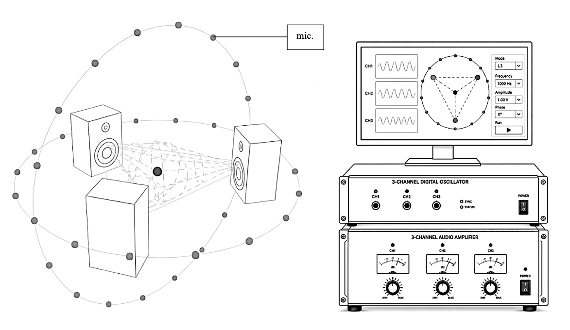
12.3 Similarity metric
Comparing two fields requires a quantity that expresses how closely they match. Without such a metric, the result would rest on visual impression alone.
Acoustic pressure is therefore measured on a grid of points around the focal region, including both amplitude and phase. The resulting two maps - one for the monolith and one for the source array - are compared point by point.
A normalized map difference relative to the maximum field value serves as one summary metric and is supplemented by spatial correlation. The threshold at which the fields are considered distinguishable is determined from the spread of repeated measurements of the same physical arrangement, that is, from the intrinsic variability of the setup.
The map comparison is supplemented by comparison of derived quantities: the position and depth of minima, pattern symmetry according to Chapter N1/10.3, and any rotating component according to Chapter N1/09.5.
This document does not specify a universal numerical threshold for field similarity. The threshold is established experimentally from the repeatability of the specific measurement setup.
A series of repeated measurements is used to determine the distribution of the metric for an unchanged physical arrangement, including variability introduced by remounting the resonator. Between measurements, the specimen is therefore removed from the holder and remounted using the same prescribed procedure. The resulting spread includes practical mounting variability that would remain hidden in a series performed without remounting.
The distinguishability threshold is established before the main comparison experiment from this distribution using a predefined statistical criterion. A practical criterion may, for example, use a multiple of the standard deviation or an appropriate repeatability interval; the specific choice, calculation method, and decision rule are recorded before the main series and remain unchanged during evaluation.
The minimum number of repetitions is selected to provide a sufficiently stable estimate of metric variability. Ten repetitions constitute the initial minimum for a pilot series; the number may be increased before the main series depending on the observed spread.
Until the threshold has been established, the metric is reported together with its measured value and variability, but without a conclusion that the two fields are identical or distinguishable. A claim of similarity without a defined threshold has no operational meaning.
12.4 What synthesis adds
Regardless of the outcome of the comparison, a multi-source arrangement has capabilities that a monolith does not, and these capabilities are informative in their own right.
Phase offsets can be varied continuously during measurement, allowing the position and organization of amplitude and phase structures to be changed electronically without mechanically moving the sources. Frequency can also be varied continuously within the operating range of the sources, whereas the monolith response is strongly constrained by its natural modal frequencies.
The arrangement also makes it possible to introduce controlled deviations deliberately. Detuning one source or shifting its phase by a known amount allows the sensitivity of the field to that deviation to be studied without manufacturing a series of monoliths with different levels of geometric precision.
The array can intentionally introduce precisely defined amplitude, phase, or geometrically equivalent deviations and track the resulting field response. In this way, it provides a controlled model for a monolith tolerance study: the electronic perturbation is known and reproducible, while an actual manufacturing deviation must be measured independently in both geometric and modal terms.
12.5 Spatial arrays
The triangular arrangement is planar. Extending it into three dimensions produces arrays in which sources point toward a common center from the vertices of a polyhedron.
Possible examples include a tetrahedron with four sources, an octahedron with six, a cube with eight, and other regular solids. More generally, extending the planar concept produces spatial arrays in which sources are directed toward a common reference region from multiple spatial directions. Suitable reference geometries may include tetrahedra, octahedra, cubes, and other regular or semiregular polyhedra.
The number and placement of sources determine the available spatial contributions, while the symmetry of the array together with their amplitude and phase relationships constrains the resulting class of synthesized field.
These arrays also provide a methodological basis for spatial configurations examined in the subsequent N3 program, which includes AURIS. Within N1, they are evaluated exclusively as measurement and synthesis arrangements.
12.6 AURISONIC
The designation AURISONIC refers to a spatial source array based on a rhombicuboctahedral frame, a polyhedron with twenty-six faces and twenty-four vertices. It corresponds to level L4 of the complexity ladder and, in its reduced-scale implementation, has an overall size of up to thirty centimeters.
AURISONIC is a modular spatial measurement array built on a rhombicuboctahedral frame with 24 vertices and 26 faces. Active sources are installed at predefined mounting positions and directed along their acoustic axes toward the center of the structure. The specific subset of active positions is recorded as part of the configuration for each experiment.
A preliminary observation under centric excitation suggested the formation of a spatial nodal structure. This is an observation made without fully recorded conditions and is listed in Chapter N1/09.10; the corresponding hypothesis is H-N1-13.
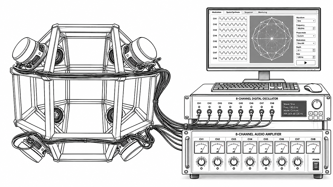
12.7 Minimum number of sources
If a multi-source arrangement can reproduce selected properties of the monolith field, the next question is the smallest number of independently controlled sources required to reproduce those properties.
The minimum number cannot be inferred solely from the dimension of the resonator's modal subspace. A two-dimensional degenerate pair represents two independent modal degrees of freedom, but it does not determine the number of physical radiators required to generate a corresponding three-dimensional acoustic map.
The experiment therefore compares arrays with different numbers of active sources. For each source count, amplitudes and phases are optimized using the same predefined procedure, and the result is evaluated with the metric defined in Chapter N1/12.3.
When a source is removed, the total excitation level is also controlled so that any degradation in similarity is not merely a consequence of reduced acoustic power. The specific active-source subset is recorded separately, because the same number of sources can generate different fields when distributed differently in space.
The minimum is defined as the smallest configuration that reproduces the predefined properties of the reference field within the established distinguishability limit. This is hypothesis H-N1-14.
12.8 Phase control as a common tool
Control of relative phase across multiple channels appears in several physically distinct systems within the documentation corpus: acoustic field synthesis, multi-point excitation of a monolith, and subsequent electromagnetic or spatial arrays.
The common feature is the ability to control the amplitude and relative phase of individual spatially distributed contributions. The same mathematical description does not imply the same physical mechanism. Phase-control terminology is therefore used consistently, while the physical interpretation remains specific to the particular system.
12.9 Phase accuracy and its limits
The resulting field depends on the actual amplitude and phase relationship among the individual acoustic contributions in the measurement region. The phase value set at the generator need not equal the phase of the acoustic pressure produced by a loudspeaker, because each channel includes electrical delay, the transfer function of the amplifier and transducer, and the acoustic propagation path between source and measurement point.
Before each comparison series, every channel is therefore measured independently and its complex transfer function between the digital excitation signal and the acoustic pressure at the defined reference point or region is determined. The phase setting is then corrected so that the required relative relationship is produced acoustically, not merely electrically.
After all channels are activated together, the relative phases are verified by synchronized microphone-array measurement. The phase error between the target and measured values, the timing spread among channels, and their stability throughout the series are recorded.
At higher frequencies, the same absolute timing error represents a larger fraction of the period, so synchronization requirements become more stringent. Phase error may shift, distort, or reduce the contrast of amplitude and phase structures; its specific manifestation is not assumed in advance.
These data form part of every measurement record because, without knowledge of the actual phase state of the sources, differences between fields cannot be reliably attributed to the geometry under investigation.
NON-CONTACT EXCITATION AND SENSING
A hammer strike cannot be reproduced exactly twice. This chapter examines ways to excite and read the resonator without physical contact.
13.1 Why a hammer strike is not enough
For measurement purposes, impulsive excitation has several limitations. The amplitude, time profile, and exact location of each strike vary slightly, so individual measurements require normalization to the actual applied impulse. Changing the point or direction of impact also changes the relative excitation of the modes. During the brief contact, the hammer additionally interacts mechanically with the resonator, so the excitation process is neither perfectly non-contact nor identical across repetitions.
Non-contact methods allow these parameters to be controlled more reproducibly while also enabling phase-defined excitation and sensing without adding mass to the arms.
13.2 Electrostatic excitation
An electrode placed near an arm and biased relative to it exerts an attractive force on the arm. The force is proportional to the square of the voltage, so with a purely alternating voltage and no DC component, the arm responds at twice the drive frequency. When a DC bias is superimposed with a small AC component, the electrostatic force contains a term that is linear in the AC-signal amplitude and acts at the drive frequency. For sufficiently small modulation relative to the bias, this regime can be approximated as linear excitation.
The same electrode can also be used for sensing. Motion of the arm changes the capacitance between the arm and the electrode, which can be measured. This creates a fully non-contact loop in which nothing touches the resonator.
Three electrodes positioned near the three arms can be driven with relative phases of 0°, 120°, and 240°. With an appropriate DC bias, this produces a spatially phase-progressive pattern of electrostatic force. The experiment then determines whether this excitation produces a stable rotating superposition within the degenerate modal subspace. Reversing the phase sequence reverses the direction of the progressive excitation; the test then examines whether the direction of the measured modal or field response reverses with it. These are hypotheses H-N1-15 and H-N1-16.
The spatial distribution of charged particles can be investigated as a separate visualization method for the electrostatic field; its interpretation requires control of particle charge, airflow, and electrode geometry.
High-voltage safety requirements are given in Chapter N1/18.
13.3 Magnetostrictive excitation
Ferromagnetic and certain other magnetically ordered materials change their dimensions when their magnetization state changes as a result of magnetostriction [49]. A time-varying magnetic field can therefore serve as a non-contact method of mechanically exciting the resonator.
The relationship among coil current, magnetic field, and the resulting mechanical force or deformation need not be linear; it may be affected by magnetic hysteresis, saturation, and the initial magnetization state. The excitation channel is therefore calibrated against the actual mechanical response of the arm, not merely against the applied current.
Three coils positioned near the three arms can be driven with relative phases of 0°, 120°, and 240°, creating a spatially progressive magnetic excitation pattern. Whether this pattern produces a rotating modal state of the resonator, and with what efficiency, is the subject of hypothesis H-N1-20.
The inverse magnetostrictive, or Villari, effect allows mechanical stress to alter the magnetic state of a material [50]. This effect can be used for non-contact sensing, although the practical arrangement must separate the weak measurement signal from the excitation field - for example by using a separate pickup coil, time separation of excitation and sensing, or phase-sensitive detection.
13.4 Three-channel magnetic pickup
Motion of a magnetized arm changes the magnetic flux through a pickup coil and induces a measurable voltage. The electrical signal therefore carries information about the time evolution of the motion, although its exact amplitude and phase relationship to the mechanical displacement depends on geometry, magnetization, and the transfer function of the sensing channel.
All three channels are therefore amplitude- and phase-calibrated before the experiment using the same reference motion. After correcting their relative transfer functions, the synchronized recordings can be used to determine the relative phase relationships among the arms.
The three-channel recording makes it possible to test in-phase motion, cyclic phase progression, and more general hybrid modal states. Evaluation is therefore not restricted to only two possibilities, 0°/120°/240° or 0°/0°/0°. This is hypothesis H-N1-17.
The underlying principle is established and is used in electric-guitar pickups and industrial reluctance sensors. Related inductive sensing principles are also used in magnetic and reluctance sensors; for this specific arrangement, however, both amplitude and phase accuracy are determined by dedicated calibration.
According to Chapter N1/09.3, two independent channels are sufficient for a complete description of the rotating state. The third channel serves as an internal consistency check, and agreement with the expected relationship is an independent indicator of measurement integrity.
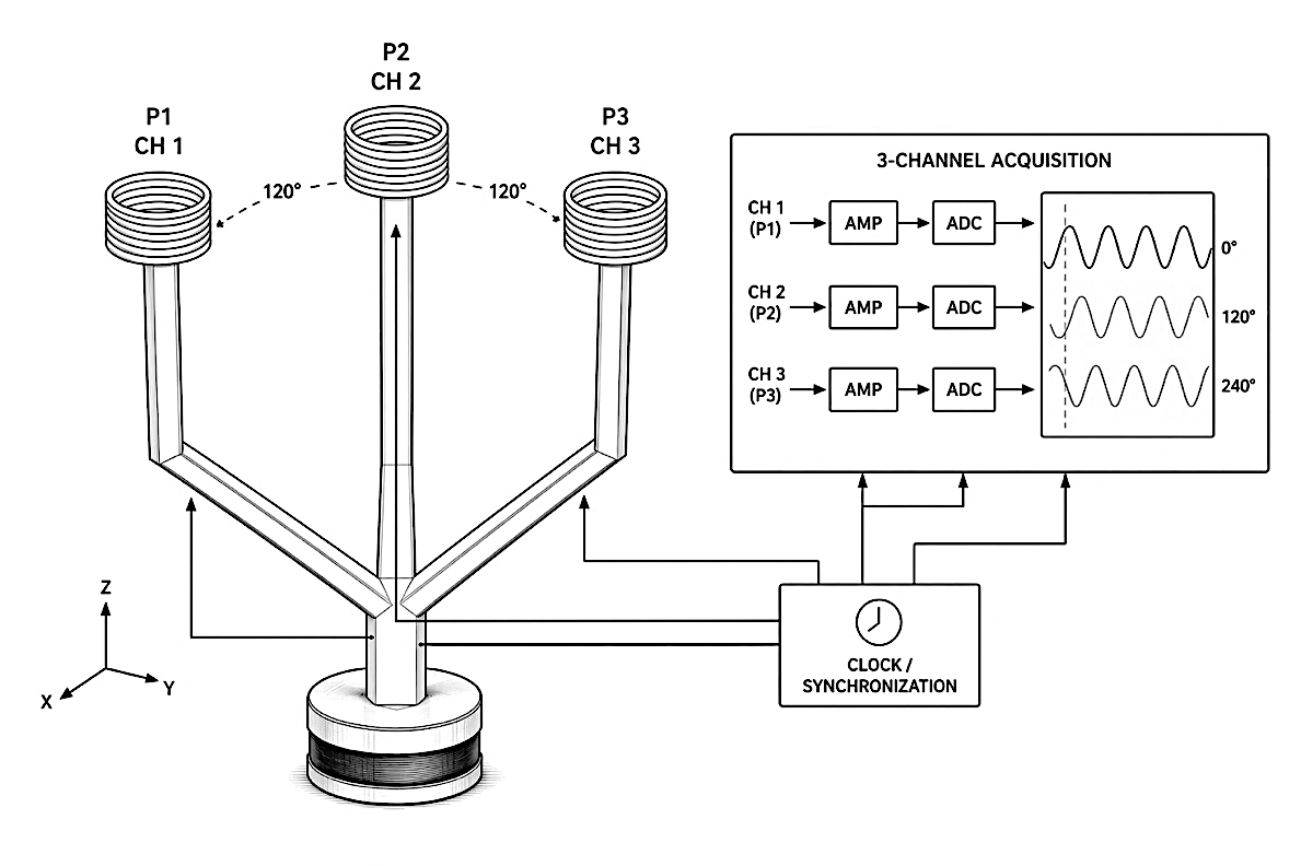
Independent verification of mechanical kinematics
Magnetic pickup provides a time-synchronized indirect record of the motion of all three arms. Its interpretation is therefore verified using an independent non-contact method, preferably laser Doppler vibrometry. The vibrometer can measure the amplitude and phase of velocity at selected points on the arms without adding sensing mass.
Where multichannel or scanning LDV is available, corresponding points on all three arms are measured and the result is compared with the three-channel magnetic pickup. A high-speed camera can supplement the measurement by directly visualizing the trajectories of the free ends; spatial reconstruction requires multiple viewing angles or stereoscopic imaging.
The resulting kinematics are classified according to the working scenarios A-C introduced in Chapter N1/09.10: predominantly symmetric motion, predominantly rotating nonsymmetric motion, or a hybrid superposition. The classification remains open to behavior that cannot be assigned unambiguously to any of these three scenarios.
Preliminary observation of arm kinematics in slow-motion video
During a preliminary visual review of slow-motion video of a three-pronged resonator with rectangular arm cross-sections, the dominant observed motion of the free arm ends was symmetric inward and outward motion corresponding to a “breathing” pattern. At the same time, individual time intervals showed deviations from perfect threefold symmetry: the projected displacement of one arm temporarily appeared weaker than that of the others, with this effect alternating among different arms.
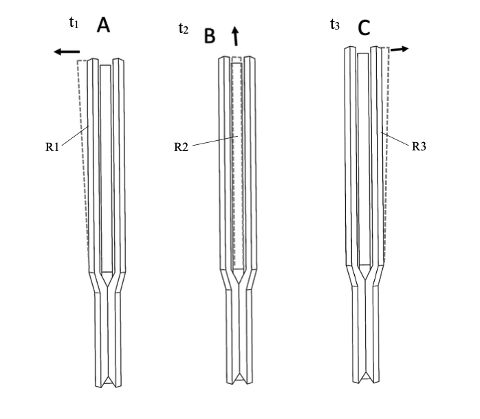
Video recording: Preliminary observation of three-pronged resonator kinematics - slow-motion recording, internal archive / online supplement, available at: https://triaural.com/MULTIMEDIA/TRIAURAL_ABC_MOVEMENT.mp4
The recording was made from an oblique lower viewing angle and without spatial calibration, so the true three-dimensional trajectories of the free ends and the precise phase relationships among the arms cannot be determined reliably from the video alone. The observation is nevertheless compatible with a superposition of multiple modal components and provides motivation for distinguishing the working scenarios A-C introduced in this chapter. The video by itself does not determine whether the motion is predominantly symmetric, predominantly nonsymmetric, or hybrid; that distinction requires synchronized spatial measurement, preferably laser vibrometry or calibrated high-speed optical imaging.
13.5 Excitation of a single arm
If one arm is excited while the other two are monitored, the intrinsic coupling of the monolith is measured - that is, how energy propagates through the body without an externally imposed phase relationship. Any phase shift measured on arms 2 and 3 is therefore not prescribed from outside.
By exciting each arm individually in sequence and synchronously measuring the response of the remaining arms, a set of mutual transfer functions is obtained. For an ideally symmetric resonator, these responses are expected to be cyclically equivalent after the corresponding relabeling rotation of the arms. A reproducible deviation may indicate geometric, material, magnetic, or clamping asymmetry and must be localized further. These are hypotheses H-N1-18 and H-N1-19.
13.6 Magnetization methods
A permanent magnet applied near the handle region can create magnetic flux passing through the central part of the resonator and dividing among the individual arms. The actual field distribution and polarity near the tips depend on geometry, material, the magnetic circuit, and magnet position and are therefore verified by measurement or a magnetostatic model.
The advantage is that the monolith remains intact and no mass is added to the tips that would alter their frequency. After the external magnetizing field is removed, remanent magnetization may remain in the material. The states before magnetization, during the applied field, and after its removal are therefore measured separately; where a return to a defined baseline is required, a controlled demagnetization procedure is used.
Instead of a permanent magnet, an electromagnet attached beneath the handle can be used, or a winding can be placed directly around the handle so that the handle serves as the core. The magnitude, polarity, and time profile of magnetization can then be controlled electronically and changed during measurement without disturbing the setup.
A continuously controlled magnetic field provides an experimental tool for testing frequency tuning according to 13.7 and controlled mode splitting according to 13.9. A winding attached to the handle adds mass and damping, so the setup is characterized both with and without the winding.
The Villari effect also underlies magnetoelectric devices addressed in document N2.
Alternatives include non-contact magnetization by an external coil or magnets attached directly to the tips. The latter option provides a stronger local field but changes the mass of the arms, which must be accounted for in evaluation.
In a symmetric magnetic arrangement, a local minimum of magnetic flux density or another characteristic field structure may arise in the central region. Its existence, position, and stability must nevertheless be determined by magnetostatic modeling and spatial measurement; they cannot be inferred from the vector symmetry of the three arms alone.
If a suitable magnetic-energy gradient is created, diamagnetic or magnetically responsive particles may show systematic redistribution. Such a distribution would constitute a magnetic visualization method analogous to particle maps elsewhere in this document, not direct evidence of a central zero-field point. This is hypothesis H-N1-24.
13.7 Frequency tuning by magnetic field
The magnetization state of a ferromagnetic material can affect its effective elastic properties and internal stress, thereby changing the natural frequencies of a mechanical resonator. The magnitude, direction, and any hysteresis of this shift depend on the material, field orientation, magnetization history, and the specific mode.
The experiment therefore tracks natural frequencies as a function of a controlled DC magnetic field while simultaneously recording hysteresis during increasing and decreasing field sweeps. If the shift is reproducible and sufficiently continuous, it may be used to fine-tune two resonators. This is hypothesis H-N1-21.
13.8 Effect of magnetization on ring-down
Magnetomechanical damping and eddy currents can change the rate at which vibration decays. Comparing the same resonator in defined magnetization states minimizes sample-to-sample differences, but requires control of remanence, magnetization history, and temperature. Changes in ring-down time, quality factor, and natural frequency are recorded. This is hypothesis H-N1-22.
If the quality factor changes with magnetization state, the time evolution and contrast of the cymatic response may change as well. This relationship is tested by correlation with the measurement described in N1/10.7.
13.9 Control of magnetic loading and mode splitting
Magnetic loading can affect the individual arms slightly differently because of geometric tolerances, nonuniform magnetization of the material, or imprecise positioning of the excitation elements. Such asymmetry can change the mode splitting of the degenerate pair and thereby affect the stability, amplitude, or time evolution of the rotating and hybrid components described in Chapter N1/09.4.
Every series using magnetic excitation or magnetization therefore includes a reference measurement with no applied magnetic field and a record of the remanent state. Without this control, a negative result could not be distinguished unambiguously from a change in modal response caused by magnetization itself.
If mode splitting can be varied controllably by magnetic field, the same specimen can be used to track how the amplitude, stability, or time evolution of the rotating and hybrid modal components changes with the splitting. Such a continuous intervention provides a stronger causal test than comparison of two different specimens. This is hypothesis H-N1-23.Δf
A useful control pair is provided by stainless steels: austenitic stainless steels are generally weakly magnetic to practically nonmagnetic in the unstressed state, whereas ferritic grades are ferromagnetic. Details are given in Chapter N1/15.
13.10 Sympathetic coupling of two resonators
Two mechanical resonators with nearby natural frequencies can couple acoustically through a shared medium. If the field produced by one resonator contains a sufficiently strong component at the receiver's resonance frequency, it can induce a measurable response in the second resonator.
A null hypothesis must be specified before measurement. The null hypothesis used here is that, for a comparable local complex acoustic field at the receiver, its linear response is independent of the identity of the distant source. The comparison with a loudspeaker must therefore match not only frequency and pressure, but also, where necessary, the relevant directional and phase characteristics of the field.
The document considers three mechanisms by which the response may differ from the null hypothesis; each is measured separately.
The first is the near field. In the near field, higher spatial components and the reactive part of the field may be more pronounced and may decay rapidly with distance. At short distances, comparison of the resonator with a control loudspeaker must therefore be based on spatial mapping rather than on a single measurement point.
The second is angular orientation. If coupling efficiency shows a reproducible periodic dependence on the relative orientation of two resonators, this indicates a directional property of the transmitting and receiving geometry that an ideal isotropic control source would not exhibit. This is hypothesis H-N1-48.
The third is the type of mode excited. If the source generates a field with measurable phase circulation and the receiver contains the corresponding degenerate or nearly degenerate pair, the experiment tests whether a directionally coupled rotating component appears in the receiver's modal response.
13.11 Measured coupling quantities
Coupling efficiency is measured over a wide range of distances. Its dependence is compared with models expected for the relevant field regions; a change in the effective decay exponent may indicate a transition between regimes, but the boundary is not defined from a single break in the curve alone.
Detuning the receiver by a known amount produces a resonance curve whose width gives the effective quality factor of the coupled system and, at the same time, the tuning tolerance.
The dependence on relative azimuthal orientation and axis inclination is also recorded, together with the rise-time constant for amplitude build-up in the receiver.
With sufficiently strong coherent coupling, normal-mode splitting into a pair of natural frequencies may occur. Observation of such splitting is strong evidence of coupling, while its absence does not rule out weaker coupling. This is hypothesis H-N1-50.
The complete series is performed twice - once with the resonator as the source and once with a loudspeaker - at the same frequency and the same pressure at the receiver location.
13.12 Reciprocity - geometry as a receiver
In linear reciprocal acoustic systems, reciprocity applies between transmitting and receiving responses under corresponding boundary conditions. The directional response of the same reciprocal element may therefore be closely related in transmission and reception.
If Triaural geometry exhibits a specific directional or modal response as a source, it is therefore justified to test the corresponding selectivity in receiver mode as well.
This can be implemented in two ways. The first uses three separate microphones spaced 120° apart and tests geometric synthesis of the receiving field. The second uses the monolith itself with sensing channels at the arms and tests its intrinsic mechanical-modal response. The results of these two implementations must not be conflated.
The measured quantities are source-direction estimation accuracy, off-axis source rejection in decibels, directional-response width, and robustness to reverberation. These are hypotheses H-N1-52 and H-N1-53.
Reciprocity closes the link to Chapter 13.10. If a source with a rotating field excites a rotating mode in the receiver, the experiment tests whether a receiver with the corresponding three-pronged modal structure responds differently to a field with measurable phase circulation than to a control field without it - in other words, whether the Triaural receiver is selectively more sensitive to a field with a rotating component than to one without it.
At this point, the boundary stated in Chapter N1/02.6 must be repeated: the term Triaural refers exclusively to the geometry of the resonator and does not refer to three-channel hearing or psychoacoustics. A receiver chapter is precisely where that confusion is most likely to arise.
HANDLE AS A WAVEGUIDE
The handle is the only part intended for direct hand contact and, at the same time, the main mechanical path between the central node, the exciter, and the operator's hand. Despite this, it remains one of the least investigated parts of the resonator.
14.1 Why a separate chapter
Throughout the preceding text, the handle is referred to as a waveguide. This is a functional claim that has not yet been supported by measurement.
Yet the handle occupies a unique position in the complete setup. Mechanical energy from FORKER may enter the resonator through the handle, and during manual use part of the mechanical vibration is transmitted through it into the hand. It is therefore a common interface for excitation, mounting, and mechanical exposure.
This chapter therefore addresses four areas: which wave families propagate in the rod, what this implies for identifying a rotating mode, how the internal stress field can be examined, and what determines transmission into the hand.
14.2 Wave families in a solid rod
In a solid cylindrical rod, three basic families of mechanical response are relevant to this chapter: longitudinal, torsional, and flexural. Multiple modes may exist within each family, and at higher frequencies more complex transverse structures may also appear.
Longitudinal waves alternate tension and compression along the axis, causing the rod to lengthen and shorten. Torsional waves twist the rod about its axis without changing its length. Flexural waves bend the rod laterally and therefore produce transverse motion.
The individual wave families have different phase and group velocities and different degrees of dispersion. Flexural waves are typically strongly dispersive, whereas the frequency dependence of wave speed may be substantially weaker over a certain frequency range for the fundamental longitudinal and torsional regimes. At higher frequencies, and when structural dimensions become comparable to the wavelength, a full modal description of the rod is required. Classical solutions for elastic waves in cylindrical rods, including the Pochhammer-Chree formulation, provide dispersion relations against which experimentally measured modes can be compared [51-54].
Under appropriate conditions, surface-localized elastic waves may also accompany the bulk modal families [55]. Their possible contribution to transmission into the hand is a separate experimental question because mechanical contact occurs at the surface of the handle.
14.3 Symmetry and mode selection
The modal state of the arms determines the time-varying forces and moments transmitted into the central node and subsequently into the handle. Their resultant combination depends on the spatial symmetry of the particular mode.
In an ideally symmetric “breathing” motion, the transverse contributions of the three arms may largely cancel at the central node. The axial, or longitudinal, component of motion may then become more prominent in the handle. The actual ratio of longitudinal, flexural, and torsional response, however, depends on node geometry and boundary conditions and must be determined experimentally.
In the nonsymmetric modal class, cancellation of transverse forces and moments generally changes. A transverse flexural component, torsional moment, or a time-varying combination of the two may therefore be transmitted into the handle. In a rotating superposition of the degenerate pair, the direction of the resultant transverse response may also change over time.
The diagnostic quantity is therefore not the mere presence of torsion, but the multicomponent mechanical response of the handle: the amplitude and phase relationships among its longitudinal, tangential, and transverse components. This signature is compared with the simultaneously measured modal state of the arms according to Chapter N1/13.4.
Hypothesis H-N1-34 tests whether this multicomponent handle response can reproducibly distinguish the working modal scenarios defined in Chapter N1/09.
Mechanical measurement of the handle and acoustic mapping of the field represent two independent levels of the experiment. Agreement in their temporal and phase behavior may support a relationship between the resonator's modal state and the resulting field; disagreement is itself a diagnostic result and requires separate explanation.
14.4 Standing wave along the handle
A finite handle is mechanically coupled at its two ends to different impedances - the central resonant node at one end and the mounting or excitation point at the other. Partial reflection of mechanical waves at these interfaces may produce standing or quasi-standing components with spatial minima and maxima of motion.
Their positions depend on handle length and cross-section, the relevant wave family, frequency, and boundary conditions. Predictions from the dispersion model are therefore compared with an experimentally measured motion map. This is hypothesis H-N1-35.
If the mounting point lies in a region of low motion for the relevant mode, mechanical loading may affect the resonance less than when mounting occurs in a region of large local displacement. The magnitude of this effect also depends on the mechanical impedance of the holder or hand. Hypothesis H-N1-38 therefore tests the dependence of quality factor and natural frequency on mounting position and mounting impedance.
14.5 Energy flow and the rotational mechanical component
A torsional wave is a mechanical state in which individual cross-sections of the handle undergo angular displacement about its axis. It therefore constitutes an unambiguously rotational component of solid-body deformation.
The presence of torsional vibration alone, however, does not determine a directional flow of angular momentum. In a standing torsional wave, two counterpropagating components may superimpose, and the time-averaged transfer of energy or angular momentum may be small or zero. In a traveling torsional wave, by contrast, directional transport of mechanical energy and angular momentum along the axis can be examined.
The experiment therefore separates local torsional amplitude from the direction of phase progression. The amplitude and phase of the tangential component are measured at multiple points along the handle, allowing standing, traveling, or hybrid torsional behavior to be distinguished.
At the same time, energy flow in the longitudinal, flexural, and torsional components is compared, and the experiment examines whether energy is transmitted predominantly through the bulk of the body or whether a significant portion of the response becomes localized near the surface.
An open question remains as to the conditions under which longitudinal, flexural, and torsional components coexist within the same excitation regime and what phase relationships exist among them.
14.6 Surface measurement
Three-axis laser vibrometry measures local surface velocity in multiple directions and allows the motion to be decomposed into axial, tangential, and transverse components. These components provide an experimental signature of longitudinal, torsional, and flexural behavior, although complex modes may contain several components simultaneously at the same point.
Strain-gauge rosettes provide direct information about local strain, but their mass, adhesive layer, and stiffness may locally alter the mechanical properties of the handle. They are therefore used as a complementary contact control for the non-contact measurement.
Holographic interferometry and speckle correlation provide full-field, non-contact deformation maps and are useful for checking whether a map reconstructed from point measurements is misleading.
A complementary method is high-speed imaging with subpixel tracking of the arm edges. After removal of common translation corresponding to holder motion, the edge positions in successive frames provide the relative motion of the arms with respect to one another.
The frame rate must be sufficiently higher than the vibration frequency being studied to reconstruct the time course with the required phase accuracy; merely satisfying the Nyquist criterion is not sufficient for this purpose. Exposure time is controlled as well, so that motion within a single frame does not produce significant blur.
14.7 Looking inside
Surface methods describe what occurs at the outer surface. They provide only indirect information about the stress distribution across the cross-section.
Photoelasticity offers a direct route. It uses the change in birefringence of a transparent material under mechanical stress. Between crossed polarizers, differences in principal stresses appear as interference fringes from which the stress distribution can be inferred qualitatively and, after calibration, quantitatively.
Time-resolved or phase-synchronized imaging makes it possible to reconstruct the evolution of the photoelastic pattern during the vibration cycle. The temporal progression of the fringes can then be used to test whether the stress structure contains standing, traveling, or hybrid components.
One limitation must be stated: a transparent model has different material constants from the metallic original, so it serves to verify the shape of the stress field rather than its numerical values. Quantitative comparison is provided by the computational model described in Chapter N1/17.
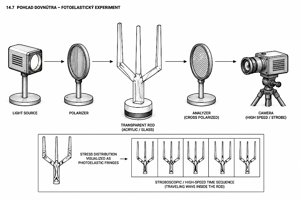
14.8 Handle geometry as a parameter
The handle is defined by its length, diameter, any taper, the geometry of its transition into the central node, and its termination.
The transition between the handle and the central node is one of the key geometric parameters because it determines the local change in mechanical impedance and thereby influences reflection, transmission, and conversion among the individual wave components.
Abrupt changes in cross-section or stiffness may increase reflection and modal conversion, whereas smoother transitions may reduce impedance mismatch within certain frequency bands. The specific effect, however, must be determined by calculation and measurement for the particular geometry.
A monolithic handle is compared with a joined handle. The joint interface may introduce additional impedance mismatch, friction, and damping. Comparing monolithic and joined implementations therefore tests the extent to which the mechanical interface changes the transfer function, mode splitting, and quality factor.
Surface finish affects surface waves and friction at the grip and is therefore recorded alongside the dimensions.
14.9 Twisted and grooved handle
A helically grooved handle is a chiral geometry because left-handed and right-handed versions cannot be made identical by simple mirror reflection without reversing handedness. Such geometric asymmetry may enable coupling between longitudinal and torsional mechanical response. The magnitude and direction of this coupling, however, depend on groove depth, pitch, number of turns, cross-section, and material and must be determined experimentally.
It follows that helical grooving may act as a converter between longitudinal and torsional waves. The geometric feature thereby becomes part of the physics of the assembly.
Hypothesis H-N1-36 tests whether, under the same excitation, a helically profiled handle exhibits a systematically different ratio of longitudinal to torsional response than a smooth control handle.
A separate control test reverses the handedness - that is, the direction of the helix. If the observed coupling is genuinely caused by chiral geometry, changing from a right-handed to a left-handed implementation should reproducibly reverse the sign of the corresponding torsional response while all other conditions remain unchanged.
14.10 Self-similar profiles
A handle profile containing geometric features repeated across multiple scales may introduce several characteristic mechanical length scales. These may influence scattering, local resonances, and mechanical-wave transmission across different frequency bands.
Whether such a profile actually creates distinct pass bands or stop bands depends on the specific geometry, material, and coupling among the individual features and must be determined from the transfer function or a dispersion model.
The experiment compares a smooth handle with a self-similarly profiled handle of the same overall length and material and as nearly the same mass as practical. The frequency-dependent transfer functions of the longitudinal, torsional, and flexural components are measured, and reproducible bands of enhanced or suppressed transmission are sought.
Historical note: fractal geometry emerged in part from the analysis of errors in data-transmission lines. During his work at IBM from 1963 to 1965, Benoît Mandelbrot found that errors did not cluster randomly but self-similarly, in a structure resembling the Cantor set.
14.11 Transmission into the hand
The hand is not a rigid support. It has its own compliance, mass, and damping, so it extracts energy from the resonator and changes its ring-down.
This behavior is covered by a standard. The mechanical impedance of the hand-arm system is defined in ISO 10068 and describes the force response of the hand to imposed vibration as a function of frequency.
Transmission into the hand depends primarily on vibration frequency and direction, grip force, contact area, grip position along the handle, and the mechanical impedance of the hand-arm system. Position relative to the local minima and maxima of motion described in Chapter 14.4 is one of the key parameters.
The transfer function between handle motion and hand response is measured at defined measurement points. Handle motion is recorded non-contact by vibrometry, while the hand response is measured, for example, using a lightweight accelerometer or optical method according to the desired level of invasiveness.
14.12 Most effective grip
The question of which grip is best has two answers, depending on the objective.
If the objective is to minimize mechanical loading of the resonator by the hand and extend ring-down, a location with low local motion amplitude for the relevant mode is a suitable candidate.
If the objective instead is to maximize mechanical transmission into the hand, a region with higher local amplitude and suitable contact mechanical impedance is a suitable candidate.
The exact optimum cannot be determined solely from the position of a node or antinode because the result also depends on vibration direction, grip force, contact area, and frequency. Hypothesis H-N1-37 therefore compares transmission and damping while the grip is moved systematically along the handle.
The documentation therefore distinguishes two separate optimization objectives: minimizing loading of the resonator and maximizing mechanical transmission into the hand.
14.13 Safety during hand-held operation
Holding a vibrating object is covered by a separate standard. ISO 5349 provides a methodological framework for measuring and evaluating vibration exposure transmitted to the hand-arm system. Long-term exposure may be associated with vascular, neurological, and musculoskeletal effects; specific action and limit values are assessed under the applicable safety regulations.
For every experiment involving manual holding, the frequency-weighted vibration level, exposure duration, grip method, and hand position are therefore recorded. Safety evaluation is kept separate from the question of the resonator's physical effect.
Operator-exposure dosimetry is developed further in Chapter N1/18. At this point, it is sufficient to state that grip position affects not only the sound but also the level of exposure.
MATERIAL BASE
What materials can the resonator be made from, and what changes as a result?
15.1 Material requirements
Material selection significantly affects natural frequencies, damping, mechanical stability, machinability, and the applicability of the magnetic methods described in Chapter N1/13. The resulting response, however, always arises from a combination of material properties, geometry, and boundary conditions.
The first requirement is low internal damping. In every material, part of the vibration energy is converted into heat, and this fraction determines how quickly the vibration decays. It is expressed by the quality factor, denoted Q.
The second requirement is repeatability. The stock material, manufacturing process, and resulting geometry must be documented so that material variability can be distinguished from manufacturing and geometric deviations.
The third requirement is machinability. The angular tolerance defined in Chapter N1/06.8 is one of the outputs of program N1; a material that cannot be machined accurately would compromise this result.
The fourth requirement is stability over time and with temperature. Resonance frequency changes with temperature, and the magnitude of this change is recorded during every measurement.
15.2 Baseline material set
The following materials form the baseline set. They are available, well documented, and span a range from high quality factor to good machinability.
- Aircraft-grade aluminum alloys - good machinability, low mass, and broad availability. Baseline material for the first series.
- Titanium and its alloys - high strength and stability, but poorer machinability and higher cost.
- Bell bronze, a tin bronze - historically used specifically for long ring-down; castable, but more difficult to machine.
- Fused silica - potentially very low internal damping and a high quality factor when appropriately fabricated; disadvantages include brittleness and demanding shaping processes.
- Brass, copper, and stainless steels - readily available and machinable, with different densities and sound velocities.
Materials with higher internal damping serve as controls for dependence of the observed phenomenon on quality factor and ring-down duration.
The following table lists approximate values taken from materials literature and catalog data. These are not values measured within this program; measured values are recorded separately, and where they conflict with tabulated values, the measurement takes precedence.
The Q and α_f values are treated as approximate ranges and are verified for the relevant material condition and frequency range before being used in the design of a specific experiment.
| Material | ρ (kg/m³) | E (GPa) | c (m/s) | Q (order) | αf (ppm/K) | Machinability |
| Aluminum alloy 6061 or 7075 | 2 750 | 70 | 5 050 | 10³ - 10⁴ | −200 to −300 | excellent |
| Titanium alloy Ti-6Al-4V | 4 430 | 114 | 5 070 | 10³ - 10⁴ | −150 to −250 | poor |
| Tin bronze, bell bronze | 8 750 | 100 | 3 380 | 10³ - 10⁴ | −250 to −350 | poorer; castable |
| Fused silica | 2 200 | 72 | 5 720 | 10⁵ - 10⁷ | +80 to +100 | brittle; grinding |
| Brass CuZn37 | 8 470 | 105 | 3 520 | 10³ | −250 to −350 | very good |
| Copper | 8 960 | 120 | 3 660 | 10² - 10³ | −300 to −400 | moderate; gummy |
| Stainless steel 304, austenitic | 8 000 | 193 | 4 910 | 10³ | −200 to −300 | moderate |
| Stainless steel 430, ferritic | 7 700 | 200 | 5 100 | 10³ | −200 to −300 | good |
Column designations: ρ is density, E is Young's modulus, c is longitudinal wave speed in a thin rod, Q is the quality factor, and αf is the temperature coefficient of resonance frequency.
Sound velocity is calculated from c = √(E/ρ) for a longitudinal wave in a thin rod so that it is derived consistently throughout the table. Different relationships apply to bulk media and flexural modes, as described in Chapter N1/16.
The quality factor is given by order of magnitude rather than as a single value. In metals, it depends so strongly on heat treatment, cold working, and surface condition that even the same material can vary by an order of magnitude or more. No authoritative universal table exists for this quantity; the decisive value is the measurement on the specific specimen.
Two rows deserve particular attention. Fused silica has a quality factor two to four orders of magnitude higher than the metals and is the only material in the table with a positive temperature coefficient because its elastic modulus increases with temperature; its resonance frequency therefore rises when heated, whereas the frequencies of the metals decrease. Copper has higher internal damping in many mechanical resonators than suitable bell bronzes. Adding tin substantially changes the alloy's microstructure, elastic properties, and damping behavior; the specific Q value nevertheless depends on composition, heat treatment, forming history, and the condition of the individual specimen.
Materials with higher internal damping, such as wood, polymers, and composites, are not included in the table. They serve as control specimens, and their tabulated properties depend so strongly on the specific specimen that a single approximate value would be misleading.
15.3 Magnetostrictive materials
The methods described in Chapter N1/13.3 require a material that changes dimensions in a magnetic field. Not every ferromagnetic material is equally suitable; the decisive criterion is the combination of effect magnitude and machinability.
- An iron-gallium alloy known as Galfenol is one of the most suitable candidates where pronounced magnetostriction and relatively good machinability are required.
- Nickel - a classical magnetostrictive material, readily machinable and inexpensive, with a smaller effect than Galfenol.
- Terfenol-D achieves very high magnetostriction, but its brittleness and difficult machining substantially complicate the manufacture of a precise monolithic resonator; it may be more suitable as an active element or layer within a composite assembly.
For magnetostrictive materials, their mechanical properties must be expected to depend on magnetization state. This is the basis of frequency tuning described in Chapter N1/13.7 and also the reason why the applied magnetic field is recorded during every measurement.
15.4 Stainless-steel control pair
To separate magnetic contributions from other effects, it is useful to have a control pair of materials with markedly different magnetic responses and otherwise as similar basic mechanical properties as practical.
Stainless steels provide such a pair. Austenitic stainless steels are generally weakly magnetic to practically nonmagnetic in the annealed state, whereas ferritic and martensitic grades are ferromagnetic.
Two geometrically identical resonators made from appropriately selected austenitic and ferritic grades can therefore serve as a practical control pair with markedly different magnetic responses and relatively similar basic mechanical parameters. They do not, however, differ exclusively in magnetism; the remaining material differences are recorded and taken into account during interpretation.
The exact grade designations and compositions will be specified after supplier availability has been verified, because actual composition varies among heats and the magnetic properties of austenitic steels also change with cold working.
The specific steel grades will be selected according to supplier availability and recorded on the specimen sheet for each piece together with the heat number and material certificate.
Permeability is taken from the material certificate and identified in the document as a supplied value under the rule in Chapter N1/15.2. A generic tabulated value for the material grade is not used because the permeability of austenitic steels changes with cold working and the delivered material may differ substantially from the tabulated value.
During incoming inspection, the value stated on the certificate is checked for consistency with the actual material. A permanent-magnet comparison serves only as initial screening. If magnetic response is experimentally critical, a quantitative permeability value or magnetization characteristic available from the certificate or an additional measurement is also recorded. Precise permeability measurement is not within the scope of this document and is not performed; the purpose of the control pair is to distinguish a magnetic material from a nonmagnetic one, not to characterize their magnetic properties.
If incoming inspection reveals a discrepancy with the material certificate, the specimen is excluded from the series and the discrepancy is recorded.
15.5 Tetrahedral topology as a manufacturing hypothesis
The 109.47° angle defined in Chapter N1/06.3 also occurs in the bonds of an sp³-hybridized carbon atom and in the silicon-oxygen tetrahedron that forms the fundamental structural unit of silicates, including fused silica.
This correspondence is not presented in the document as an argument. It is presented as a question with a measurable form: does a monolith with tetrahedral topology exhibit a different quality factor for modes associated with this angle than a body of the same material without that topology?
The numerical correspondence between the macroscopic resonator angle and microscopic bond angles does not itself constitute a physical mechanism. The experiment therefore does not test “resonance between an angle and a material,” but whether a geometrically privileged configuration made from the same material exhibits reproducibly different modal properties from nearby configurations within the same geometric family.
The primary control is a series of geometrically similar resonators in which angle φ is systematically varied around 109.47°. A simple body made from the same material and with approximately the same volume may serve as an additional reference specimen, but not as the sole control.
The hypothesis was independently proposed by two external readers of the document, which increases its value as a suggestion originating outside the team. This is hypothesis H-N1-55.
15.6 Comparing topologies from the same stock
The question of whether a four-pronged resonator behaves differently from a three-pronged resonator can be addressed using an unusually clean measurement arrangement.
Both specimens are manufactured from the same stock piece, in the same production series, on the same machine, and measured using the same metrology. Using the same parent stock substantially reduces material variability between specimens, although local microstructure, residual stress, and machining-induced differences may remain.
When different numbers of arms are compared, total mass, moment of inertia, characteristic dimensions, and natural frequencies are recorded separately. These quantities need not match exactly between topologies; their changes are therefore treated as part of the physical consequence of changing topology and are stated explicitly in the interpretation.
H-N1-56 - With the same material and comparable characteristic scale, three-pronged and four-pronged topologies exhibit reproducibly different modal structures.
15.7 Effect of manufacturing on the material
A machined material is not identical to the material in the original stock. Machining can create or redistribute residual stresses, alter the surface layer, and locally affect the microstructure.
Residual stress is one of the factors that can split the frequencies of a degenerate pair, as described in Chapter N1/09.4. Asymmetrically distributed residual stress may change the mode splitting of the degenerate pair and thereby affect the stability or relative contribution of rotating and hybrid components.
This creates a requirement for manufacturing documentation. For each specimen, the stock material and heat, machining procedure, any annealing, and surface treatment are recorded. Without these data, different behavior between two specimens cannot be interpreted reliably.
Stress-relief annealing is investigated as a separate manufacturing variable. Comparing annealed and unannealed specimens makes it possible to determine how strongly the thermal history of manufacturing affects modal properties; the effect cannot be attributed exclusively to stress relief without controlling for other microstructural changes.
15.8 Specimen series
The measurements described in this document require a specimen series that allows individual influences to be separated. The series has five branches.
- Material branch: identical geometry manufactured from different materials.
- Tolerance branch: the same material with a controlled angular deviation according to Chapter N1/06.8.
- Topology branch: different configurations manufactured from the same stock piece.
- Control branch: a pair of stainless steels and a two-pronged resonator as a comparison source.
• Scale branch: the same configuration reduced in size so that its fundamental frequency falls within the ultrasonic range according to Chapter N1/09.12.
The scale branch has three requirements that the other branches do not. It must include at least one configuration identical to a configuration in the audible portion of the series; otherwise hypothesis H-N1-63 on scale similarity cannot be tested, because only the same configuration at two different scales can be compared. It must also contain at least two different sizes so that dependence on the ratio of characteristic dimension to wavelength can be examined rather than only a single point. Finally, it includes at least one specimen with a controlled angular deviation, allowing the sensitivity of the phase singularity to controlled symmetry breaking to be studied according to H-N1-62.
Specimens in this branch are manufactured by precision machining by an external supplier. Precision machining, or another process capable of achieving the required tolerances, is preferred for the scale branch. The suitability of a specific manufacturing process is assessed according to the material, dimensions, and required geometric accuracy.
Each specimen receives a permanent identifier and its own specimen record. The identifier is stamped or engraved on the handle at a location that does not affect arm vibration.
The number of specimens in each branch is defined as follows:
| Branch | Specimens | How the specimens differ |
| Material | 8 | identical geometry, eight materials from the baseline set |
| Tolerance | 6 | same material, controlled angular deviation from zero to the tolerance limit |
| Topology | 9 | three configurations in three implementations manufactured from the same stock piece |
| Control | 3 | two stainless steels and one two-pronged resonator |
| Scale | 6 | two sizes, one configuration matching the audible series, one specimen with a controlled deviation |
| Total | 32 |
The proposed baseline series contains 32 specimens and represents the working minimum for pilot separation of the experimental branches listed above. The final number of specimens may be adjusted after pilot measurements according to the measured variability and required statistical power. The material branch, with one specimen per material, serves as a screening step in the first phase; by itself, it cannot separate a material effect from specimen-to-specimen manufacturing variability. Candidate materials are therefore verified with replicate specimens after the initial screening.
The specimen count is reflected in budget items EQ-N1-01 for manufacturing the audible portion of the series and EQ-N1-37 for the scale branch. The manufacturing reject rate is listed separately in Chapter N1/19.7 because, with controlled angular deviations on the order of tenths of a degree, some specimens will fall outside tolerance and must be remanufactured.
15.9 Crystal orientation as a geometric parameter
The discussion so far treats the material primarily as an effectively isotropic medium whose mechanical properties can, to a first approximation, be described by a single set of elastic parameters. For polycrystalline metals, this description is often sufficient because the contributions of many differently oriented grains are partially averaged at the macroscopic scale.
A single crystal behaves differently. Its elastic properties are anisotropic and depend on direction within the crystal lattice. The same body manufactured from a single crystal can therefore exhibit a different modal response depending on how the crystal lattice is oriented relative to its geometric axes.
The TORAMID configuration presents a particularly interesting case. Its three support directions can be geometrically associated with three mutually perpendicular directions corresponding to the edges of a cube, while the central axis corresponds to a body-diagonal direction. In a cubic single crystal, an orientation can therefore be selected in which the [111] direction lies along the resonator's central axis and the three arms are aligned with the [100], [010], and [001] directions.
The [100], [010], and [001] directions are crystallographically equivalent in the cubic crystal system, and the [111] direction is a threefold rotational axis. With this alignment, the threefold symmetry of the material tensor can therefore directly coincide with the macroscopic threefold geometry of the resonator.
Unlike the purely numerical angular correspondence discussed in Chapter N1/15.5, this orientation has direct mechanical significance. Rotating the crystal lattice relative to an unchanged macroscopic geometry changes the effective elastic properties along the individual segments while the external shape of the resonator remains unchanged.
This creates a clean test of material symmetry without changing the geometry of the body.
With a deliberate rotation of the crystal lattice relative to the resonator axes, the experiment tracks changes in natural frequencies, mode shapes, and splitting of the relevant degenerate or nearly degenerate pair. Lattice orientation thus becomes a continuously adjustable material variable that can break or restore correspondence between geometric and crystal symmetry.
Hypothesis H-N1-65
For a single-crystal body with threefold geometry, the modal structure and splitting of the relevant degenerate or nearly degenerate pair depend on the orientation of the crystal lattice relative to the resonator axes. In particular, the experiment tests whether alignment of the cubic [100], [010], and [001] directions with the three arms and the [111] direction with the central axis represents a symmetry-privileged or extremal orientation.
The hypothesis does not specify in advance whether the splitting will be minimal, maximal, or correspond to another characteristic point at this orientation. The computational and experimental results will determine the outcome.
Primary computational test
Before a single-crystal specimen is manufactured, the hypothesis is evaluated using the anisotropic computational model described in Chapter N1/17.
The resonator geometry remains fixed in the model, while the elastic stiffness tensor of the selected single crystal is numerically rotated relative to it. For each orientation, the following quantities are recorded in particular:
- natural frequencies of the monitored modes,
- magnitude of mode splitting Δf,
- spatial mode shapes,
- orientation of modal axes,
- relative contribution of symmetric and nonsymmetric modal components.
The alignment [111] // central axis and [100], [010], [001] // arms is compared specifically with slightly rotated lattice orientations.
The computational sweep therefore makes it possible to determine whether a measurable crystal-orientation effect exists at all and how large an angular change is required to resolve it.
Experimental manufacture of a single-crystal specimen follows only if the model predicts a difference larger than the expected experimental uncertainty and manufacturing variability.
Experimental verification
If the computational model predicts a sufficiently large effect, single-crystal specimens with known crystallographic orientation are manufactured. The lattice orientation is verified before machining and, where possible, after machining using an appropriate crystallographic method.
At least two orientations are compared:
- reference alignment of crystal and geometric symmetry,
- a defined rotated orientation with unchanged macroscopic geometry.
The measurement includes the same modal quantities as the computational model and is performed under the same mounting, excitation, and temperature conditions.
Material candidates and limitations
Single-crystal metals in the size required for an entire resonator may be difficult and expensive to manufacture. Machining may also alter the surface layer and introduce defects or residual stresses that must be separated from the effect of crystal orientation itself during interpretation.
For soft metals such as copper, the quality factor may additionally be limited by internal damping and dislocation motion. From a practical standpoint, stiffer single-crystal materials with a well-characterized elastic tensor, such as single-crystal silicon, are therefore also suitable candidates.
This branch is included in N1 as a material-geometric hypothesis. Its value lies in the ability to vary the symmetry of the mechanical properties without changing the external shape of the resonator, thereby separating geometric and material contributions to mode splitting.
MATHEMATICAL RELATIONS
How to calculate frequency from dimensions - and exactly where the calculation ceases to be reliable.
16.1 What the model must accomplish
The purpose of the analytical model is to estimate the relationship between dimensions, material parameters, and the characteristic natural frequencies of the resonator, and to determine the sensitivity of the result to changes in individual parameters. Without such a model, every specimen would have to be manufactured and measured, which would be impractical for a series with controlled deviations according to Chapter N1/06.8.
The model must answer three questions. What frequency will a body of given dimensions have? How will the frequency change when one dimension is changed? And how precisely must a dimension be maintained for the frequency to remain within a selected tolerance?
This chapter addresses the analytical approach, that is, equations. The numerical approach, which treats the shape of the body as a whole, is the subject of Chapter N1/17.
16.2 Flexural vibration of an arm
A resonator arm behaves approximately as a beam fixed at one end and free at the other. Its flexural vibration is described by the classical theory associated with Euler and Bernoulli [ref].
The frequency of such a beam depends on four quantities: length, the cross-sectional dimension in the direction of bending, the material's elastic modulus, and its density. Their relationship has the form:
f ∝ ( h/L² ) · √ ( E/ρ )
where h is the arm thickness in the direction of vibration, L is its length, E is Young's modulus, and ρ is density. The complete equation also contains a numerical coefficient determined by the boundary conditions and the cross-sectional shape.
Two practical consequences follow from the form of this relationship. Frequency decreases with the square of length, so an arm twice as long sounds four times lower when cross-section and material remain unchanged. Frequency also increases directly with thickness, so a thinner arm sounds lower.
The square root of the ratio of elastic modulus to density has the dimensions of velocity and corresponds to the speed at which longitudinal waves propagate in the material. Within the simple Euler-Bernoulli model, the material enters the natural frequency through the combination √(E/ρ). Two materials with the same value of this ratio may therefore have similar fundamental flexural-mode frequencies for the same geometry. In a more precise model, however, the result may also be affected by additional elastic parameters, anisotropy, damping, and shear deformation.
sqrt(E/ρ)
16.3 Why the simple relationship is not enough
The relationship above applies to an isolated beam fixed to an immovable support. A resonator arm, however, is not fixed in this way - it is connected to the central node, which itself moves.
Because the arms are connected through the central node, their motion cannot be described as three independent cantilever beams. Motion of one segment changes the dynamic conditions of the others, so the natural modes belong to the complete coupled structure.
For ideal threefold symmetry of this coupled system, the relevant nonsymmetric modal class may form a two-dimensional degenerate pair according to Chapter N1/09.2. Mechanical coupling determines the specific mode shapes and frequencies, while their symmetry classification follows from the symmetry of the complete body.
The analytical relationship therefore serves as an estimate and as a guide to the direction in which a dimension should be changed. The precise value, and especially the splitting of the degenerate pair, is provided only by the numerical model.
16.4 Influence of additional dimensions
In addition to arm length and thickness, other dimensions enter the result. Their influence is smaller, but not negligible.
- Arm width perpendicular to the bending direction - in the simple Euler-Bernoulli model for bending in one principal plane, the width of a rectangular cross-section cancels from the resulting frequency. In the full model, however, it affects torsional and transverse stiffness, mass distribution, and coupling to the central node.
- Shape and size of the central node - determine the stiffness of the connection and therefore the degree of coupling.
- Handle length and diameter - change its mass, mechanical impedance, and intrinsic wave behavior, thereby affecting the boundary conditions of the central node and the positions of motion minima and maxima according to Chapter N1/14.4.
- Angle φ according to Chapter N1/06.1 - changes the direction in which the arm acts on the node and therefore changes the distribution of forces.
The order in which these quantities influence frequency is addressed by the sensitivity analysis in Chapter N1/17.4.
16.5 Temperature dependence
For most common metals over the temperature range considered, increasing temperature reduces the effective elastic modulus while simultaneously increasing the dimensions of the body. Both contributions therefore generally shift the natural frequency downward. The magnitude and sign of the temperature shift are material-dependent, however; fused silica, for example, may exhibit the opposite trend as described in Chapter N1/15.2.
For the simple flexural model in Chapter N1/16.2, the approximate dependence is:
f ∝ (1/L²) · √(E/ρ)
The temperature coefficient of resonance frequency is therefore not identical to the temperature coefficient of elastic modulus alone. It includes the combined effect of changes in elastic properties, dimensions, and material density. In practice, it is therefore determined experimentally for each material as the relative change in natural frequency per unit temperature.
αf = (1/f) · (df/dT)
where αf is the temperature coefficient of resonance frequency, f is the monitored natural frequency, and T is temperature. Over a small temperature interval, the change can be approximated linearly:
Δf/f ≈ αf · ΔT
In comparative measurements, not only room temperature but also the temperature of the resonator itself, or of a sufficiently close reference point, is recorded after thermal equilibrium has been reached. In measurements comparing the frequencies of two specimens or tracking the splitting of a degenerate pair, thermal drift may be comparable to the difference being measured.
The resonator temperature is therefore recorded together with frequency in every measurement. In comparative series, specimens are allowed to equilibrate to a common temperature before measurement, and the temperature coefficient for the relevant material is verified experimentally. Approximate values are given in Chapter N1/15.2.
16.6 Splitting of the degenerate pair
Splitting of the degenerate pair, denoted Δf, is one of the key quantities in this document because it directly characterizes the degree to which degeneracy of the monitored modal pair is broken.
Δf = |f₁ - f₂|
where f₁ and f₂ are the natural frequencies of the two modes forming the monitored pair.
Breaking ideal symmetry can split the degenerate pair. This phenomenon is known in the dynamics of rotationally symmetric bodies [57], and the specific magnitude of the splitting can be affected by several different perturbations: angular deviation, unequal arm length or thickness, nonuniform residual stress, material anisotropy, magnetic loading, or asymmetric mounting.
For small symmetry perturbations, the splitting can, as a first approximation, be expected to vary smoothly with the magnitude of the perturbation. In some regimes, the leading term of this dependence may be approximately linear, but the specific form depends on the type of perturbation and the modal structure and must be determined by measurement or numerical modeling.
The tolerance study in Chapter N1/06.8 therefore tracks Δf as a function of controlled geometric deviation, while the numerical model in Chapter N1/17.4 makes it possible to separate the influence of individual parameters. The analytical model primarily provides sensitivity and order-of-magnitude estimates; the precise Δf is determined from modal analysis and the experimental spectrum.
In interpretation, Δf is not evaluated in isolation. Quality factor, resonance-peak width, mode shapes, and the amplitude and phase decomposition of motion according to Chapters N1/09 and N1/13 are recorded simultaneously. This makes it possible to distinguish frequency splitting itself from a change in damping or from a transition among symmetric, nonsymmetric, and hybrid modal behavior.
16.7 Scaling
For geometrically similar bodies made from the same material and under dynamically similar boundary conditions, natural mechanical frequencies in a linear elastic model scale approximately inversely with the characteristic dimension. If all dimensions of the body are increased by a factor s, the corresponding natural frequencies change by approximately a factor 1/s.
L → sL ⇒ f → f/s
This rule makes it possible to design one geometry and manufacture it at multiple scales with predictably shifted natural frequencies. It applies, however, to mechanical similarity of the body and does not by itself guarantee complete similarity of the radiated acoustic field.
When different scales are compared, the relevant dimensionless parameters must be preserved or at least recorded. The basic parameter is the ratio of the characteristic source dimension D to the acoustic wavelength λ, or the equivalent wave parameter:
D/λ
kD = 2πD/λ
where k is the acoustic wavenumber. Similarity may additionally be affected by quality factor, material losses, fluid loading, medium viscosity, mounting method, and other boundary conditions.
Hypothesis H-N1-63 therefore tests scale similarity, not absolute scale invariance. If the same type of modal and phase organization appears at different scales after the relevant dimensionless parameters are taken into account, this will support the interpretation that the mechanism under study is a geometric-modal property of the system. If similarity breaks down, the difference is interpreted as information about a physical parameter not preserved by simple scaling.
The scale branch of the experimental series is defined in Chapter N1/15.8, and the transition into the ultrasonic range is described in Chapter N1/09.12.
16.8 TRIAURAL Calculator
The relationships in this chapter are implemented in the TRIAURAL Calculator. From entered dimensions and material parameters, the tool estimates characteristic natural frequencies within the selected analytical model and also allows the inverse calculation of an approximate dimension for a required frequency.
Analytical results are always identified in the tool as estimates. A Triaural resonator does not exactly satisfy the conditions of an isolated straight beam with ideal boundary conditions; the arms are mechanically coupled through the central node, and the handle forms an additional dynamic element. Precise natural frequencies and mode shapes are therefore provided by the numerical model in Chapter N1/17 and subsequently by experimental measurement.
The tool is published as open-source software together with the document. For each model, its range of validity, assumptions used, and comparison of calculated values with measurements on already manufactured specimens are stated. The user therefore receives not only the resulting value but also information about the empirically determined deviation of the analytical estimate.
Flexural vibration of a cantilever beam
fₙ = (μₙ² / 2π) · (κ / L²) · √(E/ρ)
where fₙ is the natural frequency of the nth flexural mode, L is the beam length, E is Young's modulus, ρ is density, κ = √(I/A) is the radius of gyration of the cross-section, and μₙ is the dimensionless eigenvalue parameter determined by the boundary conditions [54]. For an ideal fixed-free beam, approximately:
μ₁ = 1,875 μ₂ = 4,694 μ₃ = 7,855
For higher modes, approximately:
μₙ ≈ (2n - 1)π/2
The designation μₙ is used deliberately to avoid confusion with the geometric parameter β introduced in Chapter N1/06.5 or with the acoustic wavelength λ.
Radius of gyration of the cross-section κ
| Cross-section | Characteristic dimension | κ = √(I/A) |
| Circular | diameter d | d/4 |
| Square | side a | a/√12 ≈ 0.2887a |
| Rectangular | thickness h in the direction of vibration | h/√12 ≈ 0.2887h |
| Annular | outer diameter D, inner diameter d | √(D² + d²)/4 |
Longitudinal vibration of a thin homogeneous rod
For a rod with the same type of boundary condition at both ends - free-free or fixed-fixed - the ideal one-dimensional model gives:
fₙ = (n / 2L) · √(E/ρ) n = 1, 2, 3, …
For a fixed-free combination, quarter-wave modes occur:
fₙ = ((2n - 1) / 4L) · √(E/ρ) n = 1, 2, 3, …
The actual boundary conditions of the Triaural resonator handle do not correspond exactly to either of these ideal cases. The relationships above therefore serve as reference limits and a first estimate.
Positions of nodes and antinodes
The positions of nodes and antinodes are determined from the mode-shape function of the specific mode and the actual boundary conditions. In higher modes, internal nodes are not uniformly spaced. For the resonator handle, their positions are determined numerically and subsequently verified by vibrometric measurement according to Chapter N1/14.
The analytical relationships above apply to idealized straight rods with constant cross-section. A Triaural resonator does not satisfy these conditions: its segments emerge from a common node at spatial angles, their cross-section may vary along their length, and the handle has its own dynamic response. The analytical model therefore serves for a first estimate, an order-of-magnitude check, and sensitivity guidance. Precise values are provided by the numerical model in Chapter N1/17 and verified by measurement.
COMPUTATIONAL MODEL AND VALIDATION
A model can predict what will happen before anything is manufactured. It cannot, however, replace measurement - and this chapter explains why that distinction matters.
17.1 Role of the chapter
The computational model addresses what the analytical relationships in Chapter N1/16 cannot: the behavior of the complete body, including coupling, asymmetries, and mounting conditions.
Four principles define the role of the model in program N1, and they apply without exception.
- The model is used for prediction and for determining the order of measurements. It is not a tool for eliminating measurement.
- An unvalidated model is not a result. Modeling and measurement proceed as parallel branches and are used to check one another.
- A discrepancy between model and measurement is a publishable result. It indicates that some assumption, input parameter, boundary condition, or physical mechanism in the model does not correspond to the experiment and must be identified.
- A computational model can rule out a particular state only within the physical assumptions, geometry, material parameters, and boundary conditions that it contains. A negative model result is therefore not presented as general proof that a phenomenon is impossible in the real system.
For example, if modal analysis for a particular geometry shows that no relevant degenerate or nearly degenerate pair exists within the frequency band under investigation, this is a valid negative result for that model. The next step is to test the sensitivity of the result to material parameters, geometry, mounting, and numerical settings and then compare it with experiment.
The model therefore does not determine what physics in general “allows,” but what a particular mathematical representation predicts for a particular experiment.
Sensitivity analysis can show which parameters influence the result most strongly.
17.2 Modal analysis
Modal analysis determines the natural frequencies of the body and the associated mode shapes. The body is divided into a large number of small elements, the relationships between force and deformation are formulated for each, and the resulting system is solved as an eigenvalue problem.
For program N1, three outputs are essential: the natural-frequency values, the individual mode shapes, and above all whether the frequency range under investigation contains a nonsymmetric modal class forming a degenerate or nearly degenerate pair as described in Chapter N1/09.2.
This pair is the subject of Chapter N1/09.2. The model can determine whether it exists, what its shape is, and at what frequency it occurs - exactly what the measurement then tests.
The output also includes the frequency difference within the pair. In an ideally symmetric mathematical model, the relevant degenerate pair is expected at the same natural frequency. Numerical discretization can nevertheless introduce a small apparent splitting, so mesh-convergence and symmetry-preservation checks are performed before physical symmetry perturbations are introduced.
Only splitting that remains stable under mesh refinement and changes reproducibly when a specific symmetry perturbation is introduced is interpreted as a property of the modeled body.
17.3 Harmonic analysis
Modal analysis tells us which modes the body has. It does not tell us what happens under a particular excitation.
That is the purpose of harmonic analysis. An excitation force is applied in the model at the location where FORKER acts on the body, with a specified frequency and amplitude, and the steady-state response is calculated.
The result shows which modes are excited under the given forcing and how strongly. This matters because the existence of a mode does not mean that it will be excited; the outcome depends on where and how energy is introduced.
The harmonic model also includes damping, because damping determines the amplitude and width of the response around resonance. The damping value is first estimated from the experimentally measured quality factor or ring-down and is then entered as a separate model input.
Harmonic analysis also makes it possible to test the three-phase excitation described in Chapter N1/13.3 before it is physically constructed. By applying three spatially defined harmonic forces with relative phases of 0°, 120°, and 240°, the model can test which amplitude and phase combination of modes such ideal mechanical excitation produces. Particular attention is given to whether a rotating superposition of the degenerate pair emerges. For comparison with the magnetostrictive experiment, the calibrated relationship between electrical coil excitation and the actual mechanical force described in Chapter N1/13.3 is then used.
Harmonic analysis describes the steady-state linear response. Impulsive excitation, ring-down evolution, transitions between modal states, or possible nonlinear effects require time-domain or nonlinear analysis and cannot be inferred automatically from the harmonic solution.
17.4 Sensitivity analysis
Sensitivity analysis answers which parameter influences the result most strongly. The first step uses local sensitivity analysis, in which individual parameters are varied separately around the reference geometry. This yields a derivative or relative sensitivity of the monitored quantity to each parameter.
The most influential parameters are then examined jointly so that their interactions can be captured. For manufacturing tolerances, a statistical dispersion simulation may also be added, in which geometric and material deviations are generated according to measured or manufacturing distributions.
For program N1, the primary monitored quantity is the splitting of the degenerate pair. The question is therefore which asymmetry separates it most effectively.
There are several candidates, and their ranking is not obvious in advance: deviation of the angle between arms, differences in arm length, nonuniform thickness, the geometry of the transition into the central node, asymmetric mounting, and residual stress from manufacturing according to Chapter N1/15.7.
The result has a direct practical consequence. If, for example, thickness uniformity proves more important than angular accuracy, this changes both manufacturing requirements and specimen inspection.
Sensitivity analysis also predicts the tolerance curve from Chapter N1/06.8, allowing the two to be compared point by point.
17.5 Surrounding acoustic field
The preceding analyses describe the solid body. The field generated by the body in air requires an additional step.
Surface velocities calculated by the harmonic analysis can be used as boundary conditions for calculation of the acoustic field around the resonator. The output is the complex acoustic-pressure distribution and, depending on the selected model, other field quantities in space.
This calculation can directly predict the amplitude and phase structure of the field described in Chapters N1/09 and N1/10. Comparison with a cymatic pattern is an indirect test and requires a separate coupling model linking the acoustic field, liquid, vessel, and free surface.
The model therefore makes it possible to record the expected result before measurement. A prediction written down in advance is what distinguishes an experiment from a demonstration.
17.6 Known limitations of the model
The model requires inputs that are not known exactly, and this must be acknowledged before a discrepancy with measurement appears.
- The elastic modulus of a particular specimen differs from the tabulated value and varies between material heats.
- Residual stress after machining can only be estimated approximately.
- Damping is entered into the model as a coefficient, and its value is initially determined from ring-down measurement.
- The boundary condition at the mounting point is notoriously one of the most difficult parts of this type of problem to model. A real fixture is neither perfectly rigid nor perfectly free.
Expected accuracy is not assigned as a universal percentage but is determined empirically from the validation series. Fine splitting of the degenerate pair, however, is precisely the quantity most sensitive to the aspects the model knows least well.
The following procedure therefore applies:
Model validation is separated from model calibration.
During calibration, uncertain input parameters - for example effective elastic properties, damping, or the mechanical impedance of the mounting - are refined using a predefined subset of specimens. The range of parameters that may be adjusted in this way, together with the agreement criterion, is defined before calibration.
After calibration, these parameters are frozen. The model is then tested on an independent validation set of specimens that were not used in calibration. Agreement on the validation set is the decisive measure of the model's predictive capability.
Only after successful validation is the model used to predict properties of geometries or specimens that have not yet been manufactured.
17.7 Tools and openness
The calculations can be performed using open tools, so repeating them does not require a paid software license. This is as important for replication as publishing the data.
The input files, element mesh, material parameters, and computational scripts are therefore published together with the results. Without them, the calculation cannot be reproduced and reporting it would have the value of a claim rather than a result. The solver version and settings, element type, convergence tolerances, and mesh-generation method are also recorded with the input files. When a calculation is repeated, a difference may arise from numerical settings rather than from the physical model alone.
Convergence is assessed not only by natural frequency but, for critical tasks, also by mode shape, splitting Δf, and selected local quantities in the central-node region.
Publication also includes the mesh density and how the result changes as the mesh is refined. This is a standard control indicating whether the result is a property of the body or a property of the computation.
17.8 Budget item
The computational model has its own budget line. It includes specialist time for modal analysis, computational resources, and validation measurements, without which the model has no meaningful output.
It is listed together with the other items in Chapter N1/19, and its inclusion in the budget is part of the principle that research begins with secured financing.
Tools are specified by class rather than by a particular software version. The reason is practical: a version written into the document becomes outdated within a year, whereas the class of tool and its requirements remain valid. Specific versions are recorded in the protocol for every run and published with the result according to Chapter N1/17.7.
An open finite-element tool capable of modal and harmonic analysis is used, together with a mesh generator that allows controlled refinement around the node and a results-processing environment with a scripting interface. For the acoustic field around the body, a solver capable of coupling the elastic body to the surrounding medium is used.
The scope of the validation series follows the specimen series defined in Chapter N1/15.8. The model is calibrated on a predefined calibration set consisting of the material and tolerance branches, fourteen specimens in total. After the calibrated parameters are frozen, predictive performance is evaluated on the topology and scale branches, fifteen specimens in total, none of which enter calibration. This separation is required so that agreement between model and measurement constitutes independent verification of predictive capability.
The control branch is used for separate verification of material and magnetic controls and is not included in calibration or in the model's primary validation score.
The budget item includes specialist time for modal analysis under EQ-N1-26 and computational resources under EQ-N1-25 and EQ-N1-30. Software licenses are not budgeted because open tools are used.
17.9 Computational infrastructure
The program generates data at a scale that cannot be processed continuously by hand. Outputs include multichannel recordings, laser-vibrometer data, high-speed-camera footage, crystal-image analysis, and computational models, together with measurement protocols, procedural notes, and documentation. The volume of image and audio records exceeds the volume of numerical data by several orders of magnitude.
The node therefore acquires its own computational infrastructure with locally operated machine-learning and generative-AI models. Its role is to preprocess and classify records, transform measurements into forms that can be compared across series, prepare material for documentation, and support research coordination, including work with text, tables, images, and audio.
Local operation is used for three reasons. Unpublished measurements do not leave the facility. Computation does not depend on the availability or terms of an external service, which matters in a multi-year program. And the procedure can be repeated, because every output created with AI assistance records the model identity and weights, inference-environment version, relevant generation parameters, version of the input template or prompt, and the preprocessing procedure used. If an output is to be reproducible, knowing only the model name is not enough. With an external service, the underlying model may change without notice, breaking repeatability just as surely as changing a measurement instrument would.
Models with open weights are operated locally. Closed models whose weights are not published cannot be run locally; the capability gap between the best open and best closed models is not concealed in this document and is treated as a given constraint.
The setup includes three budget items:
- EQ-N1-30, inference server with multiple compute accelerators and sufficient memory for open-weight models.
- EQ-N1-31, rack enclosure with backup power and cooling.
- EQ-N1-32, network infrastructure and storage for multimedia data.
The setup also prepares the infrastructure for possible future integration with the AURIS multiresonance chamber described in document N3. This integration is not implemented within node N1, and no N1 budget item depends on it; it is mentioned so that the infrastructure is not designed in a way that would later prevent such integration.
The operating costs of this setup - electricity, cooling, and external technical support - are listed as separate lines in Chapter N1/19.7. Under continuous operation, these costs are not negligible, and hiding them within facility rent and utilities would distort the true cost picture.
Results produced with AI assistance are subject to the same epistemic register as all other claims in the document according to Chapter N1/01.3. An interpretation proposed by a model does not become a result without verification. AI is not used as an authoritative decision-maker when classifying a hypothesis. It may propose analyses, detect candidate patterns, or prepare supporting material, but the decisive output must remain traceable to measured data and a defined analytical procedure.
SAFETY, DOSIMETRY, AND ETHICS
Before anything is put into use, it must be known what it does under controlled conditions. This chapter comes before application, not after it.
18.1 Why safety comes before application
The resonator is an object that may be held in the hand, placed in contact with the body, and operated in close proximity to a person. It is therefore capable of transmitting acoustic or mechanical energy into the user's body, regardless of how strongly the user is able to perceive that exposure.
This chapter therefore does not appear at the end of the document as an add-on, but before considerations of application. Its purpose is to define what must be measured and documented before the resonator is made available to anyone outside the research team.
The purpose of this chapter is not to demonstrate benefit. It is to characterize exposure, identify known risks, verify compliance with applicable safety criteria, and state the uncertainties that remain open.
18.2 A claim of effect is also a claim of risk
This principle is fundamental to the entire document and is stated as follows: if a device can change something in the body, it can also change it in an undesirable direction.
The consequence is inconvenient for anyone claiming that a product has a physiological effect. Such a claim also asserts that the device is physiologically active and therefore creates an obligation to demonstrate that its use is safe.
Every claim of physiological effect therefore also creates a requirement to characterize dose, exposure mechanism, and possible adverse effects.
This determines the position of program N1. Until it is documented how and at what intensity the field acts on tissue, no physiological effect is claimed and the device is not made available to the public.
At the expected operating levels, serious harm is not considered likely, but this assumption does not replace dosimetric measurement or monitoring of physiological response.
A controlled human-exposure study is therefore considered a natural part of the safety process. Physical dosimetry can determine the acoustic and mechanical exposure to which a person is subjected, but by itself it cannot establish whether a physiological response occurs at that exposure level.
Within N1, a controlled safety exposure-physiology study is therefore performed, focusing on acute and delayed responses to a precisely defined dose. Its purpose is not to demonstrate health benefit or therapeutic efficacy. Its purpose is to determine whether the exposure produces a reproducible physiological change, identify any adverse events, and establish the conditions under which further research can be conducted safely.
Each exposure is therefore paired with physical dosimetry and a predefined set of physiological and subjective indicators. Status is monitored before exposure, during exposure, immediately afterward, and, where specified by the protocol, at delayed time points. Unexpected events are recorded regardless of whether they are initially considered likely to be related to the exposure.
Temporal sequence alone is not considered evidence of causality. An individual observation may generate a hypothesis that can subsequently be tested using a controlled and, where possible, blinded procedure.
Expanded investigation of biological mechanisms, long-term physiological adaptation, health benefit, or clinical efficacy belongs to document N3. N1 establishes the safety and dosimetric foundation for that work.
18.3 Three exposure pathways
For dosimetry, three exposure situations are distinguished and measured separately. Although they may be combined in a specific use case, each represents a different pathway of energy transfer and requires its own method of characterization.
- Airborne exposure - acoustic exposure acting primarily on the auditory system and body surface.
- Contact through the handle - mechanical vibration transmitted into the hand and hand-arm system.
- Direct-contact exposure - local mechanical transfer into a specific site on the body.
Confusing these situations is a source of incorrect conclusions. Sound-level measurement does not characterize contact exposure, and vibration measurement at the handle does not characterize the complete acoustic field. The individual components are therefore measured and reported separately before their combined exposure is evaluated.
18.4 Airborne exposure
Sound pressure level is measured at locations corresponding to the exposed person's head position and recorded over time. The measurement chain must be suitable for the frequency range under study and, for measurements in the audible range, meet the requirements of IEC 61672-1 for sound level meters [58]. The standard defines two accuracy classes; Class 1 is the more stringent and corresponds to item EQ-N1-05.
Noise exposure and its relationship to the risk of hearing damage are evaluated according to the applicable standards and legal requirements in force in the country where the facility operates, including ISO 1999 [59] and relevant European or national requirements.
At minimum, level, spectral composition, exposure duration, distance from the source, source orientation, and measurement-point position are recorded. The immediate vicinity of the arm tips is also mapped separately because the local level may differ substantially from the value at the head position.
For measurements extending into the low-frequency or infrasonic range, evaluation does not rely solely on A-weighted level. An unweighted or otherwise appropriately frequency-resolved spectrum is also recorded so that low-frequency components are not suppressed by the weighting curve used.
18.5 Contact transmission to the hand
Holding a vibrating object constitutes a separate mechanical exposure. ISO 5349-1 [60] specifies the method for evaluating vibration transmitted to the hand and arm, while ISO 10068 [61] describes the mechanical response of the hand-arm system. ISO 5349-1 does not define a range within which vibration injury can be ruled out, so values derived from the standard are not treated as an absolute safety boundary.
Long-term exposure to hand-transmitted vibration can damage vascular, neurological, and musculoskeletal structures. In N1, contact exposure is therefore recorded even when an individual measurement is brief.
Acceleration at the handle surface is measured in three axes, together with its spectrum and the frequency-weighted value according to the relevant procedure in the standard. Holding duration, grip position, grip force, excitation method, and specimen used are also recorded.
Grip position affects transmitted dose according to Chapter N1/14.12. The same resonator held near a mechanical minimum and in a region of larger motion amplitude may produce different exposures. Grip position is therefore part of every measurement protocol.
18.6 Transmission into the body during direct contact
When the resonator is placed directly against the body, a local contact exposure occurs that differs from hand holding in the point of energy entry, contact area, and mechanical impedance of the tissue.
ISO 2631-1 [63] provides a methodological framework for whole-body vibration, but it cannot automatically be used as a limit for localized point contact with the resonator. For local contact, the actual acceleration and its spectrum, contact force, contact area, orientation, exposure time, and anatomical site are therefore recorded.
Within N1, transmission into deeper tissue is first characterized using a mechanical phantom or another controlled tissue model. Human measurement is performed only under an approved exposure protocol according to Chapter N1/18.12.
Contact with bone may create a different and more efficient pathway of mechanical transmission than contact with soft tissue alone and is therefore evaluated separately. Application near the head, cervical spine, major blood vessels, or other sensitive regions is not performed until a protocol for such exposure has been defined and professionally reviewed.
18.7 Mechanisms to be examined or excluded
The following mechanisms represent possible pathways by which mechanical or acoustic exposure could produce biological effects. Their inclusion does not imply that they occur with the Triaural resonator. Each is evaluated according to the actually measured dose and the scope of the specific experiment.
- Heating by absorption - its magnitude depends on intensity, frequency, exposure duration, and the properties of the exposed medium. N1 does not assume its magnitude in advance; any temperature change is determined by measurement according to Chapter N1/11.9.
- Cavitation - its occurrence depends primarily on acoustic-pressure amplitude, frequency, liquid properties, and the presence of nucleation sites. At the expected operating amplitudes, it is not considered a likely mechanism, but as power is increased its absence is verified experimentally.
- Mechanotransduction - cellular response to mechanical stimulation is an established biological phenomenon, but N1 neither assumes nor specifies a relationship between a particular Triaural exposure dose and cellular response. If investigated, it belongs in a separate biological protocol.
- Vestibular response - under certain conditions, mechanical or acoustic exposure may cause dizziness, nystagmus, nausea, or impaired balance. Such a response is recorded as an adverse event and is grounds for immediate termination of exposure.
- Low-frequency mechanical response of the body - at operating regimes in the range of a few to tens of hertz, resonant or amplified mechanical responses of individual body regions may occur. This question does not concern the normal audible operating regime but is evaluated for the low-frequency oscillatory regime described in Chapter N1/03.3.
If another reproducible biological or physiological phenomenon emerges during the research and does not fit these categories, it is not retrospectively assigned to the nearest known mechanism. It is recorded as an open observation and investigated separately.
18.8 Preliminary contraindications and exclusion criteria
Until safety has been established, intentional exposure is not performed in individuals for whom mechanical, acoustic, or related experimental exposure could present an increased risk. This list is provisional and will be reviewed by a qualified physician and an ethics committee before the first human study.
- Epilepsy or other seizure disorders, if professional review determines them to be relevant to the protocol used.
- Pacemakers, implanted defibrillators, and other active implants in experiments involving magnetic or electromagnetic elements.
- Known thrombosis, history of embolism, or another condition in which mechanical exposure could present an increased risk.
- Pregnancy, until a specific professional assessment is available for the particular type of exposure.
- Significant vestibular disorders, recurrent dizziness, or current tinnitus in protocols that may stress the auditory or vestibular system.
- Fresh wounds, fractures, postoperative conditions, or acute painful processes at the planned contact site.
A contraindication is not inferred solely from the name of a diagnosis. The decisive factor is professional assessment of the specific exposure protocol, device used, and dose.
18.9 Research-operation risks
In addition to exposure from the resonator itself, measurements involve risks associated with the laboratory equipment used. These are evaluated separately and include at least:
- High voltage during electrostatic excitation according to Chapter N1/13.2 - electric shock, stored energy in charged capacitors, electrical discharge, ozone generation, and ignition risk.
- Strong permanent magnets according to Chapter N1/13.6 - pinch injuries, sudden attraction of ferromagnetic objects, damage to implants or equipment, and projectile or fragment hazards if brittle magnets are damaged.
- Laser sources used for visualization according to Chapters N1/10.5 and N1/10.13 - eye hazard and the need for a controlled beam area.
- Discharge and plasma setups - high voltage, ultraviolet radiation, thermal loading, and pressure or mechanical hazards associated with the vessel.
- Aerosols, chemicals, and liquid samples - inhalation, skin contact, spills, and contamination of the work area.
- Moving mechanical assemblies, rotating arms, or automated positioning - impact, entanglement, or collision hazards.
For each setup, a concise risk assessment, operating procedure, list of protective equipment, and emergency procedure are prepared before first use.
18.10 Dosimetry and exposure protocol
To make data comparable across measurements, the same basic set of quantities is recorded for every series. The protocol is expanded according to the exposure situation used.
- Sound pressure level, spectrum, and time history at defined measurement points.
- Acceleration and vibration spectrum at the handle in three axes and, for local contact, at the point of application.
- Exposure duration, number of repetitions, intervals between exposures, and excitation regime.
- Temperature of the specimen, contact site, or phantom according to the type of experiment.
- Distance, position, and orientation of the resonator relative to the exposed person or phantom.
- Resonator specimen used, material, natural frequency, mounting method, and excitation regime.
- Subjective or physiological events recorded according to the approved protocol, without advance determination of causal attribution.
Measured values are published together with the other experimental data to the extent compatible with protection of personal and health information. Dosimetry allows an independent reader to assess the actual exposure without relying on verbal assurances from a manufacturer or research team.
18.11 Health surveillance of personnel
A study participant undergoes a precisely defined individual exposure. A laboratory worker may instead experience low-level or indirect exposures repeatedly over months or years. From the perspective of cumulative dose, the team may therefore represent a distinct risk group.
A cumulative exposure record is maintained for personnel, and health surveillance is implemented according to occupational-medicine principles. This does not mean using workers experimentally as test subjects; a worker is never considered an automatically available subject merely because they are present at the facility.
The surveillance program has at least three components:
- An initial professional examination before regular work with experimental sources begins, establishing baseline status.
- Periodic examinations at intervals determined by an occupational-health physician and according to the nature of the actual exposure.
- An ongoing exposure and symptom record containing the date, duration, setup used, exposure regime, and any new or unusual change in health status, even when it is not considered exposure-related at the time it is recorded.
The scope of examinations is determined by an occupational-health physician. Program N1 provides a complete description of the exposure pathways and measured doses so that the scope of surveillance can be tailored to the actual risk.
Health information is subject to protection of medical and personal data and is not published in identifiable form. Only the anonymized scope of surveillance and its methodology may be published.
If a worker develops a change that may be related to exposure or represents a health risk, work involving the relevant exposure is suspended pending professional assessment.
18.12 Ethical framework for human research
Any prospective study in which a person is intentionally exposed to the field while their physiological or subjective response is recorded for research purposes is treated within program N1 as human-subject research.
N1 may include a controlled safety exposure-physiology study. Its purpose is not to demonstrate health benefit or therapeutic efficacy. Its purpose is to determine whether a precisely defined exposure produces a reproducible acute or delayed physiological change, identify possible adverse events, and establish the conditions under which further research may proceed.
Before such a study begins, the protocol is submitted for independent ethical review according to the rules in force in the country where the facility operates. Program N1 follows this procedure even when it is uncertain whether the particular scope of measurement formally requires mandatory approval.
Participation requires informed consent. Participants are informed of the experimental nature of the device, known and unknown risks, the scope of data collection, their right to terminate exposure at any time, and the fact that the device is neither a medical device nor a validated therapeutic method.
The protocol is preregistered before data collection begins. Exposure levels, duration, number of repetitions, monitored indicators, control or sham conditions, stopping criteria, adverse-event recording procedures, and the analysis plan are specified in advance.
Each exposure is paired with physical dosimetry and a predefined set of physiological and subjective indicators. According to the protocol, status is monitored before exposure, during exposure, immediately afterward, and at specified post-exposure time points so that delayed responses can also be detected.
Exposure begins at the lowest level required to perform the measurement and is increased only according to a predefined protocol. Neither the researcher nor the participant increases the dose improvisationally on the basis of a subjectively favorable feeling or the absence of an immediate effect.
Any new or unusual physiological change is recorded as an adverse event without advance determination of causal attribution.
Temporal sequence alone is not evidence of causality. An individual observation may, however, generate a hypothesis that is subsequently tested using a controlled and, where possible, blinded procedure.
Measurement of biological response in N1 serves safety and exposure characterization. Expanded investigation of biological mechanisms, long-term adaptation, health benefit, or clinical efficacy belongs to document N3.
N1 does not assume that a measurable biological or physiological response exists. Nor does it assume that none exists. It therefore measures such responses within the scope of the safety protocol.
18.13 Procedure before access outside the research team
The resonator is not made available outside the research team for intentional use until all conditions appropriate to the relevant exposure regime have been met.
- Dosimetry according to Chapter N1/18.10 has been completed and documented.
- Measured values have been compared with the currently applicable standards, recommendations, and legal requirements for the relevant jurisdiction.
- Preliminary contraindications and exclusion criteria have been reviewed by a qualified physician for the intended mode of use.
- Instructions for use have been prepared for the device, specifying the method of use, maximum exposure regime, stopping conditions, and a clear statement of what the device is not and what has not been demonstrated about it.
- It has been documented which risk mechanisms from Chapter N1/18.7 were experimentally examined, which showed no measurable effect under the tested conditions, and which remain open.
- If the intended use includes intentional human exposure for research purposes, an approved ethical protocol according to Chapter N1/18.12 is in place.
Failure to meet any relevant condition means that the corresponding mode of use is not made available. The procedure is not shortened even if interim results appear favorable.
Compliance with currently known limits is treated as a necessary condition, not as proof of absolute safety. A limit can be defined only for a risk that has been recognized and sufficiently characterized. Exposure is therefore kept at the lowest level at which the phenomenon under study can be measured reliably and is not increased merely because a formal limit would still permit it.
The practical consequence is rigorous recordkeeping. Parameters whose significance may not yet be obvious are also recorded when they can reasonably be measured without disrupting the experiment. A recorded parameter can be reevaluated later; a missing one cannot.
For every standard, this document identifies the standard and its scope of application. Specific operational limit values are not reproduced as permanently binding numbers. When the facility is established, they are taken from the currently applicable version of the standard or legal requirement in the relevant jurisdiction and entered into the operating procedures together with the source and edition.
Acquisition of the relevant standards and professional reference materials is listed as a separate operating-cost item in Chapter N1/19.7.
18.14 Airborne ultrasound
The scale branch described in Chapter N1/09.12 moves the operating range above the threshold of audibility. This changes the safety assessment, so airborne ultrasound is evaluated separately.
For airborne ultrasound, the methodological and regulatory situation is not identical to that for ordinary audible noise. The literature and guidance use frequency-resolved exposure levels, and the evidentiary basis for some historically used limits is weaker than for standard noise exposure. N1 therefore treats such guidance as the best available reference framework, not as proof of complete safety.
Historical, national, and more recent international guidance and assessments cited in sources [64]-[66] use substantially different reference levels near the upper limit of audibility and in the higher ultrasonic range. Numerical values given in the source literature are used in this document to illustrate the sharp change in assessment across frequency bands; the binding operational limit is always taken from the currently applicable regulation or guidance in the country where the facility operates.
The decisive safety parameter is not only the carrier or fundamental frequency of the source. Nonlinear excitation or nonlinear response of the system may generate harmonics, subharmonics, difference-frequency components, or other spectral components that extend into the lower ultrasonic or audible range. Evaluation must therefore not be limited to a narrow interval around the operating frequency.
Level is evaluated in one-third-octave bands or suitably narrow frequency bands across the entire relevant range, including the upper part of the audible band. All unintended spectral components are monitored separately because they may be subject to stricter assessment than the operating frequency itself.
Safety monitoring also records acute subjective symptoms such as headache, nausea, tinnitus, a sensation of pressure in the ear, fatigue, or impaired balance. Their occurrence is not automatically interpreted as an effect of ultrasound; it is recorded as an adverse event and compared with dose, control condition, and other noise sources.
At minimum, the following measures apply to the ultrasonic branch:
- Measurement of the frequency-resolved spectrum before every series and after every change in power, geometry, or excitation regime.
- Operation in a controlled space with verified acoustic treatment for the frequency range actually used.
- Remote control and observation of the experiment from outside the primary exposure area whenever the experiment permits.
- Use of suitable hearing protection when entry during operation is unavoidable, with its actual attenuation evaluated over the relevant frequency range.
- No presence of persons who are not part of the approved measurement or operation.
- Immediate termination of exposure if vestibular, auditory, or other unexpected symptoms occur.
The contraindications in Chapter N1/18.8 apply to this branch according to professional assessment and are supplemented by any conditions for which ultrasonic or accompanying audible exposure may present an increased risk.
EQUIPMENT AND ESTIMATED COSTS
What is required for high-quality measurement, and what does it cost?
19.1 How the budget is structured
The budget is derived from the measurements described in the preceding chapters. Each item is tied to a specific experiment, so its purpose can be traced and, if the scope is reduced, it is clear which measurements would be removed.
Items are designated in the form EQ-N1-xx and are listed in the same form in the appendices, allowing them to be referenced individually.
The budget uses tax-inclusive prices as a conservative common basis; final tax treatment will be adjusted according to the legal form and jurisdiction of the facility. Price ranges are given for instruments because the difference between basic and laboratory-grade implementations can be several-fold.
The facility location has not yet been selected. For rent, utilities, health surveillance, and some services, the stated range therefore also reflects differences in price levels among possible locations. Personnel costs are currently represented by a single reference staffing model; after the location is selected, they will be recalculated according to local wage and employer-contribution conditions.
The final cost level will be refined after the location is selected according to Chapter N1/20. Until then, the budget is presented as a range and should be regarded as a rough estimate.
19.2 Scope of equipment
The facility is designed to be fully equipped and self-sufficient. Key equipment is acquired so that the progress or outcome of measurements does not depend on the short-term availability of another organization's chamber, spare capacity in another laboratory, or the willingness of a third party to provide a service.
The measurements described in this document require repetition, long series, and the ability to return to a setup after weeks without changing it. At an external or shared facility, long-term availability, configuration stability, and the ability to repeat a measurement at any chosen time cannot be guaranteed automatically. For the core research infrastructure, permanent availability is therefore treated as part of measurement quality.
The budget does not assume that key research infrastructure requiring long-term availability will be replaced by external services. Specialized one-time operations, such as precision machining, annealing, metrology, or external expert analysis, may be procured as services when owning the corresponding equipment is not economical for N1.
The budget presented in this document applies to node N1. Documents N2 and N3 have their own budgets, and their sum is outside the scope of this text.
19.3 Equipment categories
The following lists group equipment by purpose. Each item includes the chapter that requires it.
Specimen manufacturing
- EQ-N1-01 Machining of the specimen series, including the tolerance branch - Chapters N1/06.8 and N1/15.8. Contract manufacturing is assumed rather than acquisition of an in-house machine.
- EQ-N1-02 Stock material including material certificates - Chapter N1/15.
- EQ-N1-03 Heat treatment and annealing of part of the series - Chapter N1/15.7.
- EQ-N1-04 Verification metrology of dimensions and angles - Chapter N1/06.8.
Acoustic measurement
- EQ-N1-05 Calibrated Class 1 sound level meter and measurement microphone for safety dosimetry; separate measurement microphones for spatial field mapping where required - Chapters N1/12.3 and N1/18.4.
- EQ-N1-06 Multichannel measurement system with synchronous recording - Chapters N1/12.3 and N1/13.4.
- EQ-N1-07 Positioning system for grid-based field scanning - Chapter N1/12.3.
- EQ-N1-08 Semi-anechoic chamber including vibration-isolated mounting - cost depends on working volume, lower cutoff frequency, required background-noise level, and vibration isolation according to Chapter N1/20.2.
Excitation
- EQ-N1-09 Multichannel phase-controlled generator and amplifier - Chapters N1/03.3 and N1/12.2.
- EQ-N1-10 FORKER including spare parts and flexible couplings - Chapter N1/03.2.
- EQ-N1-11 Electrostatic-excitation setup including a high-voltage supply - Chapter N1/13.2.
- EQ-N1-12 Excitation and pickup coils, magnets, and controlled-current supply - Chapters N1/13.3 through N1/13.7.
Vibration measurement
- EQ-N1-13 Laser vibrometer; a three-axis implementation is preferred for full spatial kinematics, while a single-axis unit may serve as a basic or staged configuration - Chapters N1/14.6 and N1/17.6.
- EQ-N1-14 Accelerometers and strain-gauge system - Chapters N1/14.6 and N1/18.5.
- EQ-N1-15 Photoelastic-measurement setup including transparent models - Chapter N1/14.7.
Visualization
- EQ-N1-16 Laser source with light-sheet optics - Chapters N1/10.5 and N1/10.13.
- EQ-N1-17 High-speed camera and imaging setup - Chapters N1/10 and N1/14.7.
- EQ-N1-18 Cymatics station, vessels, powders, and seeding medium - Chapters N1/10 and N1/11.
- EQ-N1-19 Glass chamber for volumetric visualization - Chapter N1/10.9.
Liquid samples
- EQ-N1-20 Optical probes for dissolved gases - Chapter N1/11.6.
- EQ-N1-21 Tensiometer and viscometer with temperature control - Chapter N1/11.6.
- EQ-N1-22 Dynamic light-scattering instrument - Chapter N1/11.6.
- EQ-N1-23 Thermistor bridge and fiber-optic temperature sensors - Chapter N1/11.9.
- EQ-N1-24 Microscope and crystal-image-analysis setup - Chapter N1/11.8.
Computation, data, and processing
- EQ-N1-25 Computational workstation and data storage - Chapter N1/17.
- EQ-N1-27 Publication of data and documentation, including persistent identifiers - Chapter N1/17.7.
- EQ-N1-30 Inference server for locally operated AI models - Chapter N1/17.9.
- EQ-N1-31 Rack enclosure, backup power, and cooling - Chapter N1/17.9.
- EQ-N1-32 Network infrastructure and storage for multimedia data - Chapter N1/17.9.
Scale branch and ultrasound
Items in this group relate to the scale branch described in Chapter N1/09.12 and the safety requirements in Chapter N1/18.14.
- EQ-N1-33 Measurement microphone and preamplifier with response up to 100 kHz - Chapter N1/09.12.
- EQ-N1-34 Broadband acquisition and spectral analysis for the ultrasonic range, including one-third-octave evaluation - Chapter N1/18.14.
- EQ-N1-35 Ultrasonic transducers and excitation setup up to 200 kHz - Chapter N1/09.12.
- EQ-N1-36 Fine positioning system for millimeter-scale field scanning - Chapter N1/09.12.
- EQ-N1-37 Manufacture of scale-branch specimens by external precision machining - Chapter N1/15.8.
- EQ-N1-38 Absorptive treatment of the space for ultrasonic operation - Chapter N1/18.14.
Safety and surveillance
- EQ-N1-28 Protective equipment, laser-beam shielding, and safeguards for the high-voltage section - Chapter N1/18.9.
- EQ-N1-29 Occupational health surveillance for the facility - baseline examination and periodic checks according to Chapter N1/18.11; budgeted annually.
Safety exposure-physiology study
- EQ-N1-39 Basic physiological-monitoring setup - multiparameter recording of core physiological variables during the safety exposure-physiology study according to Chapter N1/18.12. Depending on the protocol, it allows synchronous recording in particular of heart rate and HRV, blood pressure, SpO₂, temperature, and other selected variables.
- EQ-N1-40 Sensors and consumables for human measurements - disposable electrodes, contact elements, hygiene and disinfection supplies, any single-use sensors, and other consumables required by the approved N1/18.12 protocol. The item is charged to operating costs according to the actual number of measurements.
- EQ-N1-41 Professional and ethical support for the safety exposure-physiology study - expert preparation and review of the protocol, medical collaboration, preparation of documentation for ethical review, and professional oversight of implementation according to Chapter N1/18.12. The specific scope is adapted to the legal and ethical requirements of the facility jurisdiction.
- EQ-N1-42 Costs associated with volunteer participation and any study-insurance requirements - reimbursement of reasonable participant expenses, any compensation for time, and insurance or other safeguards required by the approved protocol and facility jurisdiction. The item is used only to the extent permitted by the ethics approval and applicable rules.
Services and program items
The following items are not one-time purchases of instruments. They are listed separately from equipment so that capital and operating costs are not conflated.
- EQ-N1-26 Modal-analysis specialist work - Chapter N1/17.8. Budgeted once for the full program period as an external expert service in addition to the permanent team.
- EQ-N1-41 Professional and ethical study support - budgeted per protocol or per program according to actual scope.
- EQ-N1-42 Volunteer participation and any insurance arrangements - budgeted per program according to the approved protocol.
- EQ-N1-29 is an annual item and is included directly in operating costs according to Chapter N1/19.7. EQ-N1-40 is likewise included in annual operating costs.
Pricing of one-time items
The From and To columns state the total price for the full quantity in the relevant row, not the unit price.
| EQ | Item | Qty | From (€) | To (€) |
| EQ-N1-01 | Machining of specimen series | 1 | 18 000 | 45 000 |
| EQ-N1-02 | Stock material including certificates | 1 | 3 000 | 9 000 |
| EQ-N1-03 | Heat treatment and annealing | 1 | 1 500 | 4 000 |
| EQ-N1-04 | Verification metrology of dimensions and angles | 1 | 15 000 | 60 000 |
| EQ-N1-05 | Measurement microphone and Class 1 sound level meter | 1 | 3 000 | 12 000 |
| EQ-N1-06 | Multichannel measurement system | 1 | 6 000 | 25 000 |
| EQ-N1-07 | Three-axis positioning system | 1 | 9 000 | 35 000 |
| EQ-N1-08 | Semi-anechoic chamber | 1 | 80 000 | 300 000 |
| EQ-N1-09 | Multichannel generator and amplifier | 1 | 4 000 | 15 000 |
| EQ-N1-10 | FORKER including spare parts | 3 | 1 200 | 4 500 |
| EQ-N1-11 | Electrostatic excitation with HV supply | 1 | 3 000 | 12 000 |
| EQ-N1-12 | Coils, magnets, controlled-current supply | 1 | 2 500 | 9 000 |
| EQ-N1-13 | Laser vibrometer | 1 | 35 000 | 250 000 |
| EQ-N1-14 | Accelerometers and strain-gauge system | 1 | 4 000 | 14 000 |
| EQ-N1-15 | Photoelastic-measurement setup | 1 | 3 000 | 10 000 |
| EQ-N1-16 | Laser source with light-sheet optics | 1 | 3 000 | 12 000 |
| EQ-N1-17 | High-speed camera | 1 | 30 000 | 120 000 |
| EQ-N1-18 | Cymatics station and accessories | 1 | 2 000 | 6 000 |
| EQ-N1-19 | Glass chamber for volumetric visualization | 1 | 2 000 | 8 000 |
| EQ-N1-20 | Optical probes for dissolved gases | 1 | 4 000 | 12 000 |
| EQ-N1-21 | Tensiometer and viscometer | 1 | 8 000 | 28 000 |
| EQ-N1-22 | Dynamic light-scattering instrument | 1 | 35 000 | 100 000 |
| EQ-N1-23 | Thermistor bridge and fiber-optic sensors | 1 | 5 000 | 18 000 |
| EQ-N1-24 | Microscope and image analysis | 1 | 6 000 | 25 000 |
| EQ-N1-25 | Computational workstation and data storage | 1 | 8 000 | 25 000 |
| EQ-N1-27 | Data publication and persistent identifiers | 1 | 2 000 | 8 000 |
| EQ-N1-28 | Protective equipment and safeguards | 1 | 3 000 | 10 000 |
| EQ-N1-30 | Inference server for local AI models | 1 | 40 000 | 250 000 |
| EQ-N1-31 | Rack enclosure, power, and cooling | 1 | 5 000 | 25 000 |
| EQ-N1-32 | Network infrastructure and data storage | 1 | 7 000 | 40 000 |
| EQ-N1-33 | Microphone and preamplifier to 100 kHz | 1 | 6 000 | 25 000 |
| EQ-N1-34 | Broadband ultrasonic acquisition and analysis | 1 | 8 000 | 35 000 |
| EQ-N1-35 | Ultrasonic transducers and excitation setup | 1 | 5 000 | 20 000 |
| EQ-N1-36 | Fine positioning for scale branch | 1 | 7 000 | 30 000 |
| EQ-N1-37 | Manufacture of scale-branch specimens | 1 | 12 000 | 45 000 |
| EQ-N1-38 | Absorptive treatment for ultrasonic operation | 1 | 4 000 | 20 000 |
| EQ-N1-39 | Physiological-monitoring setup | 1 | 5 000 | 20 000 |
| One-time items total | One-time items total | One-time items total | 395 200 | 1 686 500 |
The stated prices are working estimates classified as class O and class P according to the budget appendix: class V denotes a supplier's public price list, class P a quotation requested from a supplier, and class O an estimate based on comparable products. Most items are currently class O. Before contractual procurement, each major item is updated using a current quotation or otherwise documented price source.
Items EQ-N1-30 through EQ-N1-32 constitute the computational infrastructure for locally operated AI models according to Chapter N1/17.9. The range for the inference server reflects differences among possible implementation classes and will be recalculated before procurement according to the hardware then available.
The two largest items, chamber EQ-N1-08 and vibrometer EQ-N1-13, account for a substantial part of the upper equipment-budget limit. Their prices depend mainly on chamber parameters and on whether a single-axis or three-axis vibrometer is acquired.
Pricing of services and program items
| EQ | Item | Period | From (€) | To (€) |
| EQ-N1-26 | Modal-analysis specialist work | per program | 20 000 | 60 000 |
| EQ-N1-41 | Professional and ethical study support | per protocol/program | 5 000 | 20 000 |
| EQ-N1-42 | Volunteer participation and any insurance arrangements | per program | 2 000 | 10 000 |
| One-time/program services total | One-time/program services total | One-time/program services total | 27 000 | 90 000 |
* The EQ-N1-42 range is a working estimate. The actual cost will be refined only after the number of participants, ethics-body decision, insurance requirements, and facility jurisdiction are known.
19.4 Relationship to the other nodes
Part of the equipment acquired for this node can also be used for measurements under documents N2 and N3. This primarily includes the acoustically treated space, computational and recording equipment, multichannel excitation, and visualization setup.
This is stated to make clear that the budgets of subsequent nodes do not include repeated acquisition of the same instruments. The N1 budget is not reduced on this basis; this is equipment that N1 requires regardless of whether subsequent nodes are implemented.
When multiple nodes are funded together, shared items are counted only once.
19.5 Reserves
Reserves are stated separately according to the nature of the risk. Their calculation bases must not overlap unless explicitly stated, so that the same risk is not counted twice.
- Technical reserve: 10% of one-time instrument and technical-equipment costs, excluding items subject to a separate construction reserve. It covers price movement, exchange-rate risk, necessary accessories, and differences between the working estimate and an actual quotation.
- Construction reserve: 15-20% of the costs of construction and acoustic treatment of the space and chamber. The consolidated model uses 18%; the base consists primarily of item EQ-N1-08 and any directly related construction work.
- Operating reserve: 5% of planned annual operating costs before reserves already included elsewhere. It covers unforeseen operating expenditure, not expansion of program scope.
- Replication reserve: 5-8% as a restricted fund for independent repetition of a measurement with a surprising or decision-critical result. The specific base of this reserve is stated in the consolidated budget so that it is clear which experimental costs it covers.
The replication reserve is used only to verify a result according to a predefined program decision, for example by repeating the measurement with another operator, a new specimen set, or at another facility.
Unspent funds are not automatically treated as unrestricted funds for arbitrary use. They remain bound to the purpose and funding rules of the program; transfer to further research, publication of results, bonuses, or other activities is possible only to the extent permitted by the funding agreement and after the required approval and reporting.
The program does not assume that team members will personally subsidize its operation. Reasonable personnel costs and compensation for work are planned directly in the budget, not added afterward from accidentally unspent items.
An inflation provision is stated separately from reserves. The program spans several years, so prices of instruments, materials, and labor will change during its duration. For multi-year funding, the timing of procurement is therefore recorded and an appropriate published price index for the relevant category is used.
The funding party has the right to transparent reporting on the use of funds to the extent agreed by contract; this right is not interpreted as authority to interfere with scientific results or to condition continuation of individual experimental branches on their content.
19.6 Items that are easily underestimated
The following costs are easily underestimated in research projects and are therefore listed separately.
- Calibration and service contracts. The working budget estimate uses approximately 5-10% of the value of selected measurement equipment per year; this is not a universal service rate, and the final cost is taken from the specific service and calibration terms.
- General laboratory consumables outside EQ-N1-40: powders, seeding media, chemicals, electrodes, disposable sensors, contact elements, and connecting components.
- Manufacturing scrap rate. For the tolerance series, it is assumed that some specimens may fail final metrology.
- Publication costs, including open-access fees and publication of negative results. Costs for persistent identifiers and data publication are listed separately as EQ-N1-27.
- Acquisition of standards and professional reference materials required by the safety and operating framework according to Chapter N1/18.13.
- Time for documentation, anonymization, data management, and archiving. Without this work, measurements are produced that cannot later be evaluated or replicated reliably.
- Administration of the safety study, protection of personal and health data, and preparation of materials for ethical review according to Chapter N1/18.12.
- EQ-N1-29 concerns health surveillance of personnel; EQ-N1-41 concerns professional and ethical support for participant research. These items do not overlap.
19.7 Operating costs
In addition to one-time procurement, ongoing costs arise and are stated on an annual basis.
- Team personnel costs according to headcount and FTE allocation.
- Facility rent and utilities.
- Calibration, service, and consumables.
- Operation and technical support of the computational infrastructure.
- Occupational health surveillance and consumables for the safety study.
- Any bonuses beyond salary, only if consistent with funding rules and predefined criteria.
Personnel costs are stated in aggregate. A breakdown of roles, FTE allocations, and salaries forms part of the internal budget appendix; the published figure is the total annual cost including employer contributions and overhead.
The total staffing level of the working model is approximately 9.5 FTE. It includes program leadership, two senior scientists, two researchers at doctoral or postdoctoral level, a laboratory technician, program and administrative support, and a documentation and communications role. External accounting support and administration of the computational infrastructure are treated, depending on the specific contractual model, either as services or as part of operating costs.
The working payroll calculation uses a reference annual cost of €488,300 including employer contributions and overhead. After the location is selected, the staffing model will be recalculated according to local wage and employer-contribution conditions.
Calibration and service contracts in the working budget are calculated according to Chapter N1/19.6. The base is selected measurement equipment, including scale-branch instruments EQ-N1-33 through EQ-N1-36; computational infrastructure is not calibrated and its maintenance is accounted for separately.
| Item | From (€) | To (€) |
| Team personnel costs including employer contributions and overhead | 488 300 | 488 300 |
| Output-linked bonuses beyond salary | 0 | 39 100 |
| Facility rent and utilities | 14 400 | 42 000 |
| Power and cooling for computational infrastructure | 10 000 | 25 000 |
| Calibration and service contracts for measurement equipment | 16 100 | 128 600 |
| External technical support for computational infrastructure | 3 000 | 12 000 |
| Consumables | 3 000 | 12 000 |
| Manufacturing scrap rate | 1 500 | 6 000 |
| Acquisition of standards | 500 | 1 500 |
| Publication costs | 2 000 | 8 000 |
| Documentation and data archiving | 2 000 | 6 000 |
| Occupational health surveillance (EQ-N1-29) | 800 | 3 000 |
| Safety-study consumables (EQ-N1-40) | 1 000 | 5 000 |
| Operating costs total (annual) | 542 600 | 776 500 |
EQ-N1-26, EQ-N1-41, and EQ-N1-42 are not included in the annual table because they are treated as one-time or program services. EQ-N1-29 is already included in annual operating costs and must not be counted twice.
Summary of the base three-year N1 budget
| Component | From (€) | To (€) |
| One-time items | 395 200 | 1 686 500 |
| One-time/program expert services (EQ-N1-26, 41, 42) | 27 000 | 90 000 |
| Operating costs for 3 years | 1 627 800 | 2 329 500 |
| Base three-year budget before reserves and inflation | 2 050 000 | 4 106 000 |
* The summary excludes the technical, construction, operating, and replication reserves and excludes the inflation provision. These are applied only in the consolidated financial model according to their defined calculation bases. It likewise excludes N2 and N3 costs and the legal and corporate costs listed in Chapter N1/19.8.
19.8 What the budget does not include
The budget for this node includes the equipment and services required for the basic safety exposure-physiology study according to Chapter N1/18.12. It does not include equipment, personnel, or operating costs for expanded biological, mechanistic, or clinical studies aimed at health benefit or therapeutic efficacy; those belong to document N3.
The N1 budget does not include the AURIS chamber or specialized N3 infrastructure. It also does not include equipment for electromagnetic measurements, which are the subject of document N2.
It does not include the costs of establishing and administering a legal entity, legal representation, or associated fees. These are handled separately from the substantive research budget and must be included in the final funding requirement. Routine accounting and administrative support for operations is included according to the N1/19.7 staffing and contractual model.
The stated budget represents the substantive and operating financial framework of program N1. It does not include separate compensation for the founders for assuming a multi-year executive commitment associated with leading the program, possible relocation to the country of implementation, and substantial restriction of their other professional activities. The specific scope of this compensation will be established by a separate agreement before implementation begins, according to the location, legal form, duration, and scope of the commitment. Full financial coverage of this compensation is part of the conditions under which the team can assume responsibility for the program.
The budget also does not include the final cost of closing the program and facility. Before N1 is activated, a separate closure plan will therefore be prepared covering in particular personnel and contractual obligations, dismantling, relocation or retirement of infrastructure, archiving of data and specimens, termination of leases and services, and restoration of the facility to the required condition. This cost will be included in the activation funding framework after the location and legal form are selected.
The budget likewise does not include lower-cost alternatives to key equipment. If an item is acquired at a lower cost than expected or a reserve is not used, subsequent use of those funds is governed by the funding agreement and the rules in Chapter N1/19.5 and the consolidated financing chapter.
DESIGN OF THE RESEARCH FACILITY
What should a facility look like if it is to provide full-quality conditions for pilot research of reference value?
20.1 What the facility must support
The facility must support several activities with different technical and safety requirements: precise acoustic and vibration measurement, optical and liquid experiments, work with specimens and data, experiments involving high voltage and strong magnets, and controlled human safety exposure according to Chapter N1/18.12.
These activities are separated spatially or temporally according to the degree of mutual interference and risk.
The design is therefore based on separation into functional zones. Their size and equipment follow from the measurements described in the preceding chapters; nothing is included in the facility without a direct link to a specific task. The design presented here is conceptual. Exact dimensions and technical solutions depend on the available premises and will be determined when the site is selected.
20.2 Acoustically treated space
Measurement of a free or approximately free acoustic field requires an environment in which reflections from room boundaries are sufficiently suppressed and characterized over the frequency range under study. Otherwise, the microphone records a superposition of the resonator field and the room response.
Three levels are considered, differing in complexity and cost.
- Anechoic chamber - all boundaries, including the floor, are acoustically treated. It provides the cleanest conditions and is the most expensive option.
- Semi-anechoic chamber - the reference solution proposed for N1. Its suitability for individual measurements depends on the operating frequency range, lower cutoff frequency, and required accuracy of spatial mapping.
- Acoustically treated room with absorptive elements on the walls - suitable for comparative measurements in which the quantity of interest is the difference between two setups rather than an absolute field value.
For every measurement, the operating frequency range over which the room meets the required conditions is stated. The designation “anechoic” or “semi-anechoic” is not treated as a property valid at all frequencies.
The decisive parameter is not only absorption but also background-noise level. A resonator excited at low amplitude may produce a field weak enough to be masked by street noise or building services.
Background level is therefore recorded at the time of measurement and reported together with the result. Measurements are scheduled for periods with the lowest background level whenever other conditions permit.
The space must also be isolated from building vibration. Vibrations from corridors, elevators, or traffic can propagate through the structure into the support and from there into the resonator; a microphone may not detect them, but a vibrometer will.
20.3 Measurement station
The core of the facility is the station at which the resonator is mounted and sensors move around it.
Resonator mounting is one of the critical elements. The fixture extracts energy and changes ring-down according to Chapter N1/14.4, so it is designed for repeatability and its influence is measured separately. The same specimen mounted twice must produce the same result.
The positioning system allows the field to be sampled on a grid within a defined volume around the resonator and the monitored field region according to Chapter N1/12.3. Positioning accuracy is reported together with the measured maps because it determines the finest spatial structure that can be resolved.
The station also includes a mounting arrangement for three sources used in L3 measurements according to Chapter N1/04, with adjustable spacing and inclination and with their positions and orientations documented in a common coordinate system.
20.4 Optical and liquid station
Measurements according to Chapters N1/10 and N1/11 require a darkened space, a stable camera position, and access to samples without vibration.
The station includes an optical table, or at minimum a vibration-damped platform, a calibratable camera mount at a defined position relative to the imaged region, and a controlled laser-beam area with shielding according to Chapter N1/18.9.
Volumetric visualization requires ventilation because glycerol mist accumulates in an enclosed space. Ventilation is switched off or isolated during the measurement itself if airflow would affect the tracer, and the space is ventilated in a controlled manner after the measurement.
The liquid section has its own workbench with a water supply, space for thermostating samples, and a designated location where samples remain undisturbed during exposure.
20.5 High-voltage and magnet zone
Electrostatic excitation and work with strong magnets are assigned to a dedicated, separated, and clearly marked area.
There are two reasons. The first is safety according to Chapter N1/18.9. The second is that a strong magnetic field may affect magnetically sensitive measurement instruments, certain data devices, and other nearby equipment, while also presenting a mechanical hazard from loose ferromagnetic objects.
The zone includes lockable magnet storage, a discharge circuit for capacitors in the high-voltage section, ventilation for cases in which high-voltage operation generates ozone or other reaction products, and access restrictions for persons with active or magnetically sensitive implants according to the risk assessment of the specific setup.
20.6 Specimens and recordkeeping
The specimen series described in Chapter N1/15.8 contains many pieces that differ by small geometric deviations, including angular differences on the order of tenths of a degree, and several cannot be distinguished reliably by visual inspection.
High-voltage and strong-magnet setups are operated according to separate procedures and do not need to be active simultaneously.
Every intervention that changes the magnetic or thermal state of a specimen is recorded as part of its history.
Storage is therefore part of the facility design. Each specimen has its own designated location, permanent identifier, and record sheet maintained from manufacture through retirement.
The specimen-storage area is maintained at stable temperature because resonance frequency changes with temperature according to Chapter N1/16.5. A specimen brought from cold storage is allowed to equilibrate before measurement, and the equilibration time is recorded.
Magnetized and non-magnetized specimens are stored separately to prevent mix-ups or unintended magnetization of a control specimen.
20.7 Data infrastructure
Measurements generate large volumes of records, particularly high-speed video and multichannel time-series data.
The facility includes primary working storage, a separate backup, and the computational infrastructure described in Chapters N1/17.9 and N1/19.3. Critical data are not stored on a single physical device only.
Raw data are stored separately from processed outputs and must not be overwritten by subsequent processing.
The system also defines how measurement conditions are attached to each record. A recording without documented conditions becomes unusable over time, so it is stored together with the protocol in machine-readable form.
20.8 Controlled human-exposure station
The safety exposure-physiology study described in Chapter N1/18.12 uses the acoustically treated Zone 1 as a controlled exposure station. In N1, this is not a clinical room or therapeutic facility. The station is used exclusively for safety characterization of precisely defined exposure and for simultaneous recording of physiological response.
During measurement, the participant remains in Zone 1 without the operator present unless the approved protocol requires otherwise. Measurement, excitation, and physiological recording are controlled from a separate workstation outside the acoustic measurement space. This reduces the influence of another person on the acoustic field while preserving stable measurement conditions across exposures.
Visual supervision is provided by one or more fixed cameras with sufficient coverage of the participant and experimental setup. The station includes two-way voice communication and the ability to stop excitation immediately from the control workstation. The participant also has a clearly accessible means of signaling or terminating exposure immediately.
The space includes a position for a seated participant or, where required by the protocol, a recumbent participant, the physiological-monitoring setup EQ-N1-39, and mechanically defined reference points or a positioning system that allows the distance, orientation, and position of the resonator relative to the body to be reproduced. Participant and device positions are recorded as part of the exposure protocol.
A large observation window between the exposure and control spaces is not considered a required component of N1. If used, its acoustic influence must be included in room characterization. Camera-based supervision is therefore preferred because it allows more uniform acoustic treatment of the walls.
Excitation and measurement equipment are controlled remotely wherever possible. This also makes it possible to implement sham or blinded conditions without visual contact between the participant and the operator or with the source configuration.
The operator remains immediately available for intervention throughout the exposure, and the access route to the participant remains unobstructed; remote control does not mean leaving the participant unattended.
No other experimental activity takes place in Zone 1 during human exposure. High-voltage devices, strong magnets, open laser beams, aerosols, or other hazardous setups must not be active at the same time unless explicitly required by the specific approved protocol and covered by separate safety measures.
Participant health and identifying information are stored separately from ordinary experimental data according to Chapter N1/18.12. Camera recordings are treated as personal data and retained only to the extent required by the approved protocol.
20.9 Operating conditions
Temperature in the measurement space is kept stable and recorded continuously. This requirement follows directly from Chapter N1/16.5 because thermal drift in precise modal measurements may be comparable to the small frequency differences being monitored.
Humidity is also recorded. It affects damping in wooden and polymer specimens and changes conditions in liquid measurements.
Atmospheric pressure is also recorded for acoustic measurements when its variation may affect the speed of sound or comparability of spatial maps.
Ventilation must be designed so that airflow does not disturb the measurement. During volumetric visualization, ventilation is switched off while recording, and this condition is documented because it also affects the thermal control described in Chapter N1/10.12.
Server infrastructure must not disturb the thermal stability of specimen storage.
20.10 Construction stages
The facility is not built all at once. Individual components are established in an order corresponding to the timeline in Chapter N1/21.
- Stage one - measurement station, mounting, excitation, and recording. An acoustically treated room is sufficient.
- Stage two - optical and liquid station and visualization.
- Stage three - high-voltage and magnet zone.
- Stage four - semi-anechoic chamber as the reference acoustic facility for N1. Its final parameters are determined from the first measurements of background noise, the operating frequency range, and the required spatial measurement range. Earlier experiments may proceed in an acoustically treated room before the chamber is completed.
This sequence allows pilot measurements to begin before the facility is fully completed. Results from the first series are used to refine the chamber's technical parameters, not to decide whether the chamber will be acquired for the full N1 program.
Controlled human-exposure measurements do not begin automatically once Zone 1 is technically complete. They are activated only after physical and dosimetric characterization of the relevant exposure regime and after the ethical and safety conditions in Chapters N1/18.10 and N1/18.12 have been met.
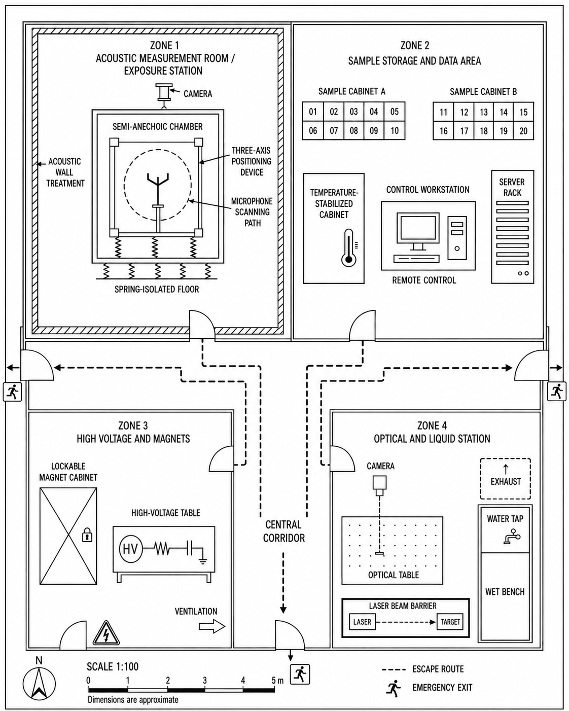
Proposed research-facility floor plan
TIMELINE
In what order, and why in that order.
21.1 How the plan is structured
The plan divides the program into phases that are linked by results, not merely by time. Progression to the next phase occurs only once the outcome of the preceding phase is known.
The phases represent scientific and operational milestones, not individual funding rounds. The primary N1 financial model assumes that the full planned scope of the program is secured through a one-time restricted contribution or donation before the main implementation begins. The funds are then managed within the approved N1 budget according to the actual course of the research.
Decisions to continue, modify, or terminate a specific research branch are made on the basis of measurement results and the methodological criteria of the document, not on the need to repeatedly request release of another portion of the budget from the funding party.
This arrangement allows the program to be scientifically closed or redirected at a phase boundary without making research decisions dependent on ongoing external financing. Unused funds remain managed according to the purpose of the funding and the applicable agreement.
21.2 Phase F0 - preparation
The purpose of this phase is to bring the facility to a state in which measurements can be performed and to obtain reference values against which subsequent results will be compared.
- Establishment of the first facility stage according to Chapter N1/20.10.
- Calibration of the measurement chain and determination of background level.
- Manufacture of the specimen series according to Chapter N1/15.8, including manufacturing documentation for each specimen.
- Construction of the computational model and its calibration on the predefined calibration set according to Chapter N1/17.6.
- Baseline health examinations of personnel assigned to regular experimental operation according to Chapter N1/18.11.
- Preparation of the safety exposure-physiology protocol, its preregistration, and submission for independent ethical review according to Chapter N1/18.12.
- Preregistration of protocols for Phase F1 measurements.
The output of the phase is a functional basic facility, a documented specimen series, a calibrated computational model with predictions recorded in advance, and completed protocols for Phase F1.
21.3 Phase F1 - primary validation
This phase answers whether the resonator contains the relevant degenerate or nearly degenerate pair and what amplitude and phase organization of motion develops among the arms.
- Physical and dosimetric characterization of the planned exposure regime according to Chapters N1/18.3 through N1/18.10.
- After dosimetric, ethical, and safety requirements have been met, the basic safety exposure-physiology study according to Chapter N1/18.12.
- Modal measurement and comparison with the model; verification of the existence of the degenerate pair.
- Three-channel magnetic pickup according to Chapter N1/13.4.
- Single-arm excitation and cyclic-symmetry test according to Chapter N1/13.5.
- Measurement of ring-down, quality factor, and mounting influence.
- Cymatic measurement with controls according to Chapter N1/10.4.
The decision point at the end of the phase is unambiguous. If the relevant degenerate or nearly degenerate pair does not appear even after verification of numerical convergence, experimental sensitivity, and the investigated range of geometric and boundary conditions, the modal mechanism proposed in Chapter N1/09 is unsupported for the tested configuration. The relevant hypotheses are marked as unsupported, and according to the predefined decision rule the program either moves to a modified geometry or closes this research branch.
21.4 Phase F2 - systematics
This phase converts individual observations into dependencies. It measures not one specimen but series of specimens and series of settings.
- Tolerance study according to Chapter N1/06.8, measuring splitting as a function of deviation.
- Comparison of L2 and L3 according to Chapter N1/04.5, including the similarity metric.
- Measurement of angular momentum using the torsional target and discrimination from streaming according to Chapter N1/09.6.
- Volumetric visualization with a test of spacing dependence on frequency according to Chapter N1/10.11.
- Handle measurements including the ratio of torsional and longitudinal components according to Chapter N1/14.3.
- Measurements of liquid samples including the rotation test and thermal calibration according to Chapters N1/11.4 and N1/11.9.
- Material comparison and measurement of the control pair according to Chapters N1/15.4 and N1/15.6.
The decision point at the end of the phase concerns the publication series as a whole. If the fields of the L2 and L3 arrangements cannot be reproducibly distinguished using the predefined metric and measurement sensitivity, hypotheses that assume a specific contribution of monolithic topology beyond a controlled array of separate sources lose support under the tested conditions. The program is then redirected toward properties attributable to geometry and control of separate sources.
21.5 Interim outputs
Publication does not wait until the end. After each phase, the measured data, protocols, and results are published regardless of whether they support the original expectation.
The reason is replicability. If data are published only after the program ends, no one can verify them while replication could still influence the course of the program.
The second reason is protection against unintentional adaptation. A published interim result cannot later be reformulated according to how subsequent measurements turn out.
21.6 Order of the first measurements
The following measurements are scheduled immediately after calibration. They do not require the completed chamber or the full instrument set, and their results determine the direction of the remainder of Phase F1.
| Hypothesis | Measurement | Prerequisite |
| H-N1-17 | Three-channel magnetic phase pickup from the arm tips | magnetized specimen, pickup coils |
| H-N1-18 | Excitation of one arm, sensing of the remaining two | excitation channel, synchronization |
| H-N1-19 | Cyclic-symmetry test by sequential arm excitation | same setup |
| H-N1-27 | Modal measurement and comparison with computation | vibrometer; microphone as supplementary acoustic measurement; computational model |
| H-N1-10 | Basic physical dosimetry of the exposure regime | calibrated acoustic measurement chain |
The order is not binding for the entire phase; it is binding for its beginning. If any of these measurements produces an unexpected result, the plan for the remainder of the phase is reconsidered before continuing.
21.7 What can change the plan
The plan is modified for three reasons, and in every case the change is recorded with a date and justification.
- A measurement result that changes an assumption. This is a desirable reason and one anticipated by the plan.
- An exploratory finding according to Chapter N1/01.4 that requires separate verification. The replication reserve according to Chapter N1/19.5 is intended for such cases.
- External circumstances, particularly instrument lead times and availability of external services.
Changing the plan because a result does not match expectations is not among these reasons.
21.8 Relationship between the timeline, budget, and funding independence
The primary N1 financial model assumes one-time non-repayable funding of the program, with no claim by the funding party for repayment of the contributed funds. The specific legal form of financing, restricted use of funds, and rules for their administration are defined by agreement before the main implementation begins.
Funding does not grant the funding party the right to interfere with measurement results, data interpretation, hypothesis classification, or decisions on scientific procedure. Publication of a positive, negative, or inconclusive result must not be conditional on the funding party's approval.
The timeline phases determine the sequence of procurement, experiments, and operating expenditure within an already secured budget. They do not represent separate funding rounds or require repeated approval by the funding party to continue.
Securing the full program at the outset allows equipment with long lead times to be procured sufficiently in advance while preserving the scientific team's ability to change the order of experiments according to measured results without disrupting financial continuity.
The phases are linked to the timing of procurement and operating expenditure within the already secured N1 budget. The minimum functional scope covers Phase F0 and part of F1; the target scope covers Phases F0 through F2.
At the boundary of each phase, a self-contained and publishable output is produced. If the results justify terminating or redirecting a particular branch, the work completed up to that point remains fully usable and reproducible.
Estimated duration and procurement linkage:
| Phase | Duration | Procurement in this phase |
| F0 - preparation | 9-12 months | EQ-N1-01 through 07, 09, 10, 25, 28; initiation of EQ-N1-41; preparation of EQ-N1-39; first facility stage |
| F1 - primary validation | 10-12 months | EQ-N1-11 through 20, 26, 27; EQ-N1-39 through 42 according to the approved protocol; second and third facility stages |
| F2 - systematics | 12-15 months | EQ-N1-21 through 24, 30 through 32; completion of reference chamber EQ-N1-08 |
| F3 - scale branch | in parallel with F1 and F2 | EQ-N1-33 through 38 |
| Total | 31-39 months |
Item EQ-N1-41 is activated already in Phase F0 because professional and ethical preparation of the safety exposure-physiology study must precede any human exposure. Setup EQ-N1-39 may be procured during F0, but its use with participants begins only in F1 after the G-HUMAN safety milestone has been met. Items EQ-N1-40 and EQ-N1-42 are used only according to the approved protocol and the actual scope of the study.
The F3 scale branch may technically proceed in parallel with F1 and F2, but its comparative interpretation requires reference results from the audible series. F3 data collection may therefore begin before completion of F2, while final evaluation of scale similarity is completed only after the relevant reference data have been obtained.
The base financial model uses 36 months. The working timeline spans 31-39 months; if the program exceeds 36 months, additional operating costs are funded and reported separately according to the actual extension.
G-HUMAN - safety milestone for human research: intentional human exposure is activated only after physical dosimetry of the planned regime has been completed, stopping criteria have been verified, and the required ethical approval has been obtained. This milestone is independent of whether the preceding physical results support the program's main hypothesis.
The stated duration is an estimate for the team size defined in Chapter N1/19.7. The range reflects instrument lead times, which for the laser vibrometer and chamber are measured in months rather than weeks; procurement therefore begins at the start of the phase rather than during it.
The F3 scale branch may technically proceed in parallel with F1 and F2, but its comparative interpretation requires reference results from the audible series. For this reason, F3 data collection may begin before completion of F2, while final evaluation of scale similarity is completed only after the relevant reference data have been obtained.
HYPOTHESES
A consolidated list of everything this document states as an open research item, together with what would resolve each item.
22.1 Two types of questions
The document uses two types of research items, each with a different nature and role.
A hypothesis asks whether something is true. It has a testable criterion and a falsification criterion, so it can be shown to be wrong. It is designated H-N1-xx.
An open question asks how or why something occurs. It cannot be falsified because it does not assert a proposition; it seeks an answer. It is designated Q-N1-xx.
Both types are necessary and serve different purposes. A hypothesis gives the document testability and protects it from being reshaped to fit the outcome. An open question allows investigation of observed phenomena that do not yet have an explanation and cannot be reduced meaningfully to a yes-or-no form.
An open question has one mandatory element: a defined output. It states what the result will be - a map, curve, catalog, or classification. Without such an output, the question would have no boundary and there would be no way to determine when it had been answered.
22.2 Summary of hypotheses
The following table contains all hypotheses in the document in abbreviated form, together with their register and phase. The full wording, including the falsification criterion, is given in the chapter where each hypothesis is introduced. Hypothesis status is updated in the working register according to the rules of this chapter.
| ID | Abbreviated wording | Reg. | Phase |
| H-N1-01 | A toroidal rotating structure forms around the axis in the focal region. | [H] | F1 |
| H-N1-02 | Frequency is predictable using an adapted flexural model. | [H] | F2 |
| H-N1-03 | Configuration changes the spatial distribution of the field in the focal region. | [H] | F2 |
| H-N1-04 | The basic taxonomy can be extended with additional geometrically unambiguous configurations. | [H] | F1-2 |
| H-N1-05 | Four-pronged resonators have analogous field variants. | [H] | F2 |
| H-N1-06 | The resonator generates nonzero acoustic angular momentum. | [H] | F2 |
| H-N1-07 | Under selected excitation conditions, standing and rotating components coexist in the acoustic field of a Triaural resonator. | [H] | F2 |
| H-N1-08 | The cymatic pattern is a signature of source geometry. | [H] | F1 |
| H-N1-09 | The configuration can be reconstructed from a static pattern. | [H] | F2 |
| H-N1-10 | The measured exposure profile of the planned regime meets the applicable safety criteria and currently valid limits for the relevant exposure type and facility jurisdiction. | [H] | F1 |
| H-N1-11 | Contact transmission through the waveguide is measurable and quantifiable. | [H] | F1 |
| H-N1-12 | Multi-source synthesis reproduces the monolith's nodal network. | [H] | F2 |
| H-N1-13 | The rhombicuboctahedral array produces the same nodal structure. | [H] | F2 |
| H-N1-14 | A minimum number of sources exists for faithful synthesis. | [H] | F2 |
| H-N1-15 | Electrostatic excitation has lower variability than impact excitation. | [H] | F1 |
| H-N1-16 | Three-phase electrostatic excitation imposes a rotating state. | [H] | F1 |
| H-N1-17 | Three-channel magnetic pickup reveals phase progression. | [H] | F1 |
| H-N1-18 | Excitation of one arm produces a phase-shifted response. | [H] | F1 |
| H-N1-19 | The response is cyclically symmetric under sequential excitation. | [H] | F1 |
| H-N1-20 | Three-phase magnetostrictive excitation imposes a rotating state. | [H] | F1 |
| H-N1-21 | A magnetic field enables continuous frequency tuning. | [H] | F1 |
| H-N1-22 | Magnetization changes quality factor and ring-down. | [H] | F1 |
| H-N1-23 | Magnetization controllably splits the degenerate pair. | [H] | F2 |
| H-N1-24 | An inward-bent configuration produces a magnetic null. | [H] | F2 |
| H-N1-25 | Geometrically privileged configurations defined in Chapter N1/06 exhibit mutually distinguishable modal or field responses. | [H] | F2 |
| H-N1-26 | A threshold deviation exists above which the phenomenon disappears. | [H] | F2 |
| H-N1-27 | Modal analysis predicts a degenerate pair in agreement with measurement. | [H] | F1 |
| H-N1-28 | The surface pattern corresponds to Faraday instability. | [H] | F1 |
| H-N1-29 | Deposition reproduces the nodal structure of the field. | [H] | F1 |
| H-N1-30 | Pattern symmetry is linked to source geometry. | [H] | F1 |
| H-N1-31 | Exposure changes dissolved gases and surface tension. | [H] | F1 |
| H-N1-32 | A taste difference is demonstrable by a blinded test. | [H] | F2 |
| H-N1-33 | Exposure changes nucleation parameters during freezing. | [H] | F2 |
| H-N1-34 | The ratio of torsional to longitudinal components in the handle changes systematically among different modal states. | [H] | F1 |
| H-N1-35 | Node positions along the handle are predictable. | [H] | F1 |
| H-N1-36 | Helical grooving couples longitudinal and torsional response. | [H] | F2 |
| H-N1-37 | Transmission into the hand depends more strongly on grip position than on grip force. | [H] | F2 |
| H-N1-38 | Handle length changes quality factor through node position. | [H] | F1 |
| H-N1-39 | The rotating component has the character of a phase singularity. | [H] | F2 |
| H-N1-40 | Structures linked to arm positions form in the aerosol. | [H] | F1 |
| H-N1-41 | Structure spacing is inversely proportional to frequency. | [H] | F1 |
| H-N1-42 | Flow velocity increases with the square of amplitude. | [H] | F2 |
| H-N1-43 | At sufficient volume, the flow closes into a cell. | [H] | F2 |
| H-N1-44 | Exposure deposits measurable heat into the sample. | [H] | F1 |
| H-N1-45 | Thermal input differs between the Triaural and conventional source. | [H] | F1 |
| H-N1-46 | Crystallization in the field changes crystal habit and size distribution. | [H] | F2 |
| H-N1-47 | In the far field, the response is independent of source type. | [H] | F1 |
| H-N1-48 | In the near field, coupling depends on relative orientation. | [H] | F2 |
| H-N1-49 | A resonator used as the source excites a rotating mode in the receiver. | [H] | F2 |
| H-N1-50 | Strong coupling produces normal-mode splitting. | [H] | F2 |
| H-N1-51 | Splitting increases monotonically with angular deviation. | [H] | F2 |
| H-N1-52 | The Triaural receiving field has different directional accuracy. | [H] | F2 |
| H-N1-53 | The Triaural receiver is more sensitive to the rotating component. | [H] | F2 |
| H-N1-54 | A classifier assigns pattern topology above chance level. | [H] | F2 |
| H-N1-55 | At φ = 109.47°, the TETRAMID configuration exhibits a reproducibly different modal response from nearby configurations of the same C3 geometric family when material and characteristic scale are comparable. | [H] | F2 |
| H-N1-56 | With the same material and comparable characteristic scale, three-pronged and four-pronged topologies exhibit reproducibly different modal structures. | [H] | F2 |
| H-N1-57 | Two-frequency excitation of nearby modal components produces a time-varying spatial superposition whose characteristic evolution rate corresponds to the difference between the excitation frequencies. | [H] | F2 |
| H-N1-58 | EQUATOR exhibits different mechanical-energy transfer into the central waveguide than neighboring configurations of the base branch. | [H] | F2 |
| H-N1-59 | Mirror configurations with the same φ exhibit different mechanical or field responses because of the opposite axial orientation of the support arms. | [H] | F2 |
| H-N1-60 | A three-pronged resonator can, under excitation without an intentionally imposed azimuthal phase gradient, produce reproducible acoustic-field phase circulation linked to its intrinsic modal dynamics. | [H] | F2 |
| H-N1-61 | The fundamental rotating state associated with the nonsymmetric degenerate pair of a three-pronged resonator produces a phase singularity with topological charge |l| = 1, with the sign reversing when the direction of phase circulation is reversed. | [H] | F2 |
| H-N1-62 | Controlled breaking of threefold symmetry systematically changes the position, stability, or topological structure of the phase singularity associated with the rotating state. | [H] | F2 |
| H-N1-63 | For geometrically similar three-pronged resonators, the character of the modal and acoustic rotating response is preserved across different scales when the relevant dimensionless system parameters, including the ratio of characteristic dimension to wavelength, are comparable. | [H] | F3 |
| H-N1-64 | Under selected excitation conditions, the vibration of a three-pronged resonator may simultaneously contain measurable symmetric and nonsymmetric modal components. | [H] | F2 |
| H-N1-65 | For a single-crystal body with threefold geometry, the modal structure and splitting of the relevant degenerate or nearly degenerate pair depend on crystal-lattice orientation relative to the resonator axes. In particular, the experiment tests whether alignment of cubic directions [100], [010], and [001] with the arms and [111] with the central axis represents an extremal or symmetry-privileged orientation. | [H] | F2 |
22.3 Open Questions
The following questions arise from phenomena repeatedly observed during work with the devices and not yet explained. Each is stated together with the output by which it is considered answered.
| ID | Question | Output |
| Q-N1-01 | What determines the symmetry of the cymatic pattern? | map of patterns in the frequency-amplitude plane for each configuration |
| Q-N1-02 | How does the pattern evolve during ring-down, and under what conditions does it remain spatially stable? | time-resolved record of pattern evolution from excitation to silence, with quantified stability |
| Q-N1-03 | To what extent does pattern shape depend on source material, frequency, and geometry? | comparative series across materials, frequencies, and configurations, with quantified pattern similarity |
| Q-N1-04 | What is the shape of the spatial nodal network around the resonator? | three-dimensional field map with nodes identified at several frequencies |
| Q-N1-05 | Why does the apparent sound-source position shift at some locations? | map of locations showing the effect, compared with the measured field |
| Q-N1-06 | What does sound pulsation reveal about the modal state? | time-frequency analysis of pulsation, estimate of Δf, and spatial-phase comparison with modal measurement |
| Q-N1-07 | Are the spatial nodes cross-sections of the same structure visualized by cymatics? | comparison of planar and volumetric maps under identical conditions; agreement in spacing, common rotation with the source, and matching response to frequency changes |
| Q-N1-08 | How do modal structure and the spatial field change continuously with angle φ across the base and mirror branches? | curves/matrices of monitored quantities as functions of φ and axial branch |
| Q-N1-09 | What are the temporal and amplitude contributions of the symmetric and nonsymmetric modal components during vibration of a three-pronged resonator? | time-resolved decomposition of modal components and classification according to scenarios A-C, or identification of another response pattern |
Questions Q-N1-04 and Q-N1-05 also apply to an arrangement without a monolith, namely the spatial source arrangement described in Chapter N1/12.6. They therefore do not depend on the outcome of the L2-versus-L3 comparison in Chapter N1/04.5 and remain open even if the fields of the two arrangements cannot be distinguished.
22.4 Notes on individual questions
Q-N1-02 Pattern evolution and stability
Faraday patterns can transition between states as amplitude changes. Preliminary observation [O] suggests that under some conditions the monitored pattern may persist through a significant part of the ring-down. Its temporal stability is therefore measured and quantified without assuming it in advance.
Q-N1-03 Dependence on material and frequency
According to preliminary observations to date [O], visually similar patterns have appeared with some resonators made from different materials and having different natural frequencies. The extent of this similarity has not yet been systematically quantified.
If high similarity is confirmed in a controlled series, it will become possible to investigate to what extent the dominant symmetry of the pattern is linked to source geometry and which of its properties remain sensitive to material, frequency, amplitude, and boundary conditions.
Verification requires controlled variation of the individual parameters and quantification of similarity according to Chapter N1/10.3.
Q-N1-06 Sound beating
Pulsation in the sound of a ringing resonator may arise from the superposition of two spectral components with nearby frequencies. In the simple two-frequency case, the characteristic envelope frequency is determined by their frequency difference, so the corresponding frequency splitting can be estimated from the time record.
The presence of beating alone does not determine the spatial character of the superposition. Two nearby modes may produce a standing, rotating, precessing, or more general time-varying response depending on their mode shapes, relative amplitudes, and phase.
The discriminating measurement therefore uses multiple synchronized channels located at different azimuths. It tracks not only envelope frequency but also relative phase and the spatial evolution of complex amplitude. A systematic azimuthal shift may support interpretation as a moving or precessing structure; common modulation in all directions is compatible with a standing or globally amplitude-modulated response.
At exact degeneracy, beating caused by a frequency difference disappears. This alone does not distinguish a standing state from a rotating state because both can be formed by different superpositions of the same degenerate pair. The decisive measurement is spatially and phase resolved according to Chapters N1/09 and N1/13.
Pulsation therefore provides information about the presence of nearby frequency components, not independent evidence of rotation.
22.5 Conditional hypotheses
Some hypotheses are meaningful only if a test at a lower level of the complexity ladder has been passed. The document states these dependencies in advance and commits to reclassifying a hypothesis if its condition is not met.
| Hypothesis | Conditional on | What is lost | What remains |
| H-N3-01 to 07 | L2 versus L3 (N1/04.5) | claim of specificity to the monolith | field effect as such |
| H-N1-01, 06, 07, 39 | Existence of the degenerate pair | two-mode superposition mechanism | rotation arising from another mechanism |
| H-N1-34 | Excitation of the rotating mode | interpretation of the component ratio in the handle | measurement of the components as such |
In such a case, the hypothesis is not withdrawn as a topic; it moves to unsupported status. Falsification applies to a specific claim with a specific mechanism, never to an entire field of inquiry.
A hypothesis that has moved to unsupported status or has been falsified remains in the register with that historical status. If a new mechanism, measurement method, or exploratory finding justifies another test, a new or explicitly revised hypothesis is formulated with its own identifier and a link to the original result. The original status is not changed retrospectively.
The scope of N1 is not an exhaustive list of every experiment that can be performed with the defined system. During implementation, additional exploratory branches may arise from measured results or new technical possibilities. These may include, for example, controlled mechanical rotation of the complete resonator or additional geometric variants. Such measurements are designated exploratory, documented separately, and do not retrospectively change the status or criteria of preregistered hypotheses. A substantial new mechanism or independent hypothesis is introduced only as a new versioned research item.
22.6 What remains valuable regardless of the outcome
Some program outputs do not depend on whether a rotating component of the field is confirmed. They are therefore listed separately.
- Tolerance curve of splitting as a function of angular deviation according to Chapter N1/06.8.
- Modal description of the C3-symmetric monolith, including comparison with computation.
- Comparison of three-pronged and four-pronged topologies manufactured from the same stock piece according to Chapter N1/15.6.
- Angular dependence of sympathetic coupling according to Chapter N1/13.10.
- Ratio of torsional and longitudinal components in the handle according to Chapter N1/14.3.
- Minimum number of sources required for faithful field synthesis according to Chapter N1/12.7.
- Map of cymatic and surface patterns and their dependence on experimental conditions.
- Geometric parametrization according to Chapter N1/06 and normative terminology according to Chapter N1/08.
This list forms part of the assessment of the program's scientific value. Even if the main hypothesis is not supported, the result remains a body of systematic measurements, geometric parametrizations, experimental protocols, and definitions with independent methodological and replication value.
FINANCING ANALYSIS AND OPEN OPPORTUNITY
What the research requires, under what conditions, and why it does not begin before it is funded.
23.1 What this chapter is
The preceding chapters describe what is to be measured and how. This chapter describes the conditions under which that work can be carried out.
This is not a grant application. The document is not being submitted to any agency and does not seek allocation of funds through a competitive call. It is an analysis intended to allow anyone to assess what the program requires and what it will provide in return.
The chapter is deliberately written without persuasion. Anyone considering support for the research needs numbers and conditions, not an argument for its importance; that argument is contained in the rest of the document.
23.2 The principle on which the program stands
Research begins with funding, not before it. The team's contribution to date has been exhausted and will not be extended further.
No program item, including preparatory measurements, is assumed to be work performed free of charge or financed from the team's own resources. This principle applies regardless of how inexpensive some individual measurements may appear.
The reason is practical. A program that performs part of its work without financial coverage cannot determine its true costs and cannot provide a reliable estimate for continuation.
23.3 Scope and structure
The budget is structured for one fully equipped and self-sufficient facility according to Chapter N1/19.2. It is not offered in tiers and does not contain reduced-cost variants.
The stated division into phases F0-F3 determines the timing of procurement and expenditure within the secured budget; it does not represent alternative funding levels or separate tranches.
There is a practical reason for this decision. The program depends on repeated measurements, long series, and keeping setups unchanged between measurements. A reduced scope would produce results that would later have to be repeated, and the cost of repetition would exceed the initial saving.
Reserves are included in the budget as separate items with stated rates according to Chapter N1/19.5, rather than as an unspecified surcharge. Their composition is disclosed in the same way as the rest of the budget.
The stated amount applies to node N1. Documents N2 and N3 have their own budgets.
The budget is structured for three years according to the timeline in Chapter N1/21. The following table summarizes the items stated in Chapters N1/19.3, N1/19.5, and N1/19.7.
| Item | From (€) | To (€) |
| Equipment - one-time procurement | 395 200 | 1 686 500 |
| Services - one-time over the program period | 27 000 | 90 000 |
| Operating costs for three years | 1 627 800 | 2 329 500 |
| Subtotal | 2 050 000 | 4 106 000 |
| Technical reserve, 10% of equipment | 31 520 | 138 650 |
| Construction reserve, 18% of chamber EQ-N1-08 | 14 400 | 54 000 |
| Operating reserve, 5% of operating costs | 81 390 | 116 475 |
| Replication reserve, 8% of subtotal | 164 000 | 328 480 |
| Total reserves | 291 310 | 637 605 |
| Total budget | 2 341 310 | 4 743 605 |
Inflation provision - determined according to the timing of procurement and operating expenditure and a selected public price index; in the working budget it is stated separately from the reserves.
The stated amounts are rough estimates. The lower bound corresponds to basic instrument implementations and a lower-cost location; the upper bound corresponds to laboratory-grade implementation and procurement and employment within the European Union. The difference between the two bounds is therefore substantial and will be refined only after a location is selected and specific quotations are obtained.
The stated three-year summary is the public technical and operating calculation for N1, not the final amount required to activate the program. After location-specific, legal, and organizational conditions, schedule risk, separate founder compensation, facility-closure costs, and other items that cannot yet be meaningfully priced are included, the preliminary N1 activation funding envelope is estimated at EUR 6-10 million. This is an indicative range; a precise calculation will be prepared only in negotiations with a serious prospective funding partner after the specific implementation model has been defined.
The activation envelope also includes an appropriate reserve for exploratory research appendices that may arise from program results or new technical possibilities. Their inclusion will be documented separately and must not retrospectively change preregistered hypotheses or their criteria.
23.4 What the budget includes
The budget includes equipment according to Chapter N1/19.3, operating costs according to Chapter N1/19.7, reserves according to Chapter N1/19.5, and an inflation provision for multi-year financing.
It also includes items that are often omitted from comparable budgets: instrument calibration and servicing, consumables, specimen-manufacturing scrap, acquisition of standards, publication costs including publication of negative results, and time for documentation and data archiving.
The N1 budget includes the equipment and services required for the basic safety exposure-physiology study according to Chapter N1/18.12. It does not include expanded biological, mechanistic, or clinical studies aimed at health benefit or therapeutic efficacy; these belong to N3. It likewise does not include the AURIS chamber or specialized N3 infrastructure, equipment for electromagnetic measurements that is the subject of N2, or legal and organizational setup.
23.5 Reserves and unspent funds
One item is stated separately because it is relatively uncommon in research-program budgets.
The replication reserve is a restricted portion of funds intended for independent repetition of a measurement that produced a surprising result. It is used exclusively when a measurement yields a surprising, decision-critical, or methodologically significant result that, according to predefined criteria, requires independent repetition.
Setting aside funds to verify one's own result is part of the same position applied elsewhere in the document: preregistration, publication of negative results, and predefined conditions under which a hypothesis loses support.
23.6 What the program provides
There are three outputs, and they are provided regardless of how the measurements turn out.
- Raw measured data together with protocols and measurement conditions, published after each phase.
- Documentation enabling independent replication: specimen manufacturing drawings, computational files, measurement procedures, and processing scripts.
- Geometric parametrization according to Chapter N1/06 and normative terminology according to Chapter N1/08.
The outputs that do not depend on confirmation of the main assumption are listed in Chapter N1/22.6.
The program is not conceived as a closed series of measurements. If the stated questions are answered, further questions will arise from them, some extending beyond acoustics. The program anticipates this and is structured accordingly; documents N2 and N3 are the first step in that expansion.
This is stated as a starting point, not as a prediction. The scope of any continuation depends on measurement results and cannot be quantified today.
23.7 Openness and its consequences
All results are published. The output of programs N1-N3 of the TRIAURAL project is not a commercial product. The TRIAURAL project does not sell devices derived from these programs and does not commercialize the research results. An open license or public release of the results does not, however, exclude their independent use by third parties under the terms of the applicable license and legal framework.
It follows that supporting this program does not provide exclusive rights to the results or preferential access to them. This is stated in advance so that expectations do not arise that the program cannot meet.
Openness has another consequence that is stated in advance: published results may be used by anyone, including parties with whom the project would not choose to collaborate. Control over funding is not control over the use of results. The project considers openness the correct decision even with this consequence because it protects the results from appropriation.
23.8 Form of financing
Program N1 is designed for capital funding by one financially capable funding party or a small number of such parties. It does not use a model in which gradual public aggregation of small donations is a condition for program activation.
The main implementation of N1 begins only after the entire agreed activation funding framework has been secured through binding commitments. The exact amount is determined before financing is concluded, based on location, legal form, staffing model, timeline, contractual terms, and the other items stated in Chapters N1/19 and N1/23.3.
Funding may be provided by one or more contractually coordinated parties. If multiple entities participate, their commitments must be structured so that scientific progress does not depend on the ongoing acquisition or approval of additional funding tranches.
Acceptance of financing does not create a claim for repayment of the contributed funds or a right to interfere with the direction of the research, interpretation of data, classification of hypotheses, or publication of results. The specific legal form, restricted use of funds, reporting method, and other conditions are defined contractually before transfer.
Additional support received after the base financing of N1 has been secured may be used to expand or accelerate research activities, increase replication capacity, create additional reserves, or prepare and implement the subsequent N2 and N3 programs. Specific allocation is decided according to the current status of the individual programs, their approved budgets, and the purpose for which the funds were provided.
If a funding party is interested in comprehensive support of the TRIAURAL project beyond N1, financing may be contractually divided among programs N1, N2, and N3 or reserved for their subsequent implementation. The fact that N1 is already fully funded therefore does not preclude acceptance of further support for the project.
Any small-scale support for ordinary publication or website operations, if officially made available by TRIAURAL, is separate from financing of programs N1-N3 and is not counted toward their activation funding framework.
TRIAURAL does not authorize and will not authorize third parties to organize public fundraising for programs N1-N3 or any other programs of the TRIAURAL project. Any official financing is verified exclusively through the official contact information and information published on the triaural.com domain. The TRIAURAL project expressly disassociates itself from all public collections, campaigns, or other third-party fundraising initiatives claiming to support programs N1-N3 of the TRIAURAL project or any other programs or activities of the TRIAURAL project and assumes no responsibility for them.
Transparent reporting on the use of funds is provided to the extent and at the intervals agreed by contract. This right does not authorize the funding party to approve individual experimental branches on an ongoing basis or to condition their continuation on the result obtained.
For larger transfers, payment details are verified directly between the contracting parties, and the transfer method is selected according to the security and legal requirements of the relevant jurisdiction.
23.9 Conditions the project imposes on itself
The following conditions apply regardless of who supports the program.
- Results are published, including results that do not support the original assumption.
- Protocols are registered before data collection and are not modified after data collection.
- The device is not made available outside the team until the conditions in Chapter N1/18.13 have been met.
- No therapeutic or other physiological claims are made unless supported by measurement.
- The direction of research is determined by the sequence of the complexity ladder in Chapter N1/04, not by an expected outcome.
- The project reserves the right to decline support.
- Funding does not give the funding party the right to veto publication of a positive, negative, or inconclusive result.
If support were conditional on abandoning any of the conditions above, the program would not accept it.
The right to decline support also applies when the origin of the funds, the conditions attached to their provision, or the purpose for which they are offered conflicts with the principles of this document. This assessment forms part of preparation of the agreement according to Chapter N1/23.8.
SUMMARY AND OPEN CALL
What the document establishes, what it leaves open, and an invitation to replication.
24.1 What the document establishes
The document establishes five elements that, from this point onward, are normative for the entire publication series.
- Geometric parametrization and angular relationships according to Chapter N1/06, together with the normative terminology for resonator components according to Chapter N1/08. These definitions are not redefined in subsequent documents.
- The method for labeling claims according to their evidentiary weight and the distinction between hypotheses and open questions according to Chapters N1/01.3 and N1/22.1.
- The L0-L7 complexity ladder as the reference axis for progression according to Chapter N1/04.
- The geometric taxonomy of configurations and the relationship between arm angle and inclination to the axis according to Chapter N1/06.
- The conditions under which the device may be made available outside the team according to Chapter N1/18.13.
These elements are outputs of the document regardless of the outcome of the measurements it proposes.
24.2 What the document does not claim
The negative scope stated in Chapter N1/01.5 is repeated at the end because these are precisely the statements most easily overlooked during reading.
The document does not claim that a rotating component of the field has been demonstrated. It states why its existence is hypothesized, how it could be confirmed by measurement, and what would falsify it.
The document does not claim that a specific biological or physiological response to Triaural exposure has been demonstrated. Its existence or absence is measured within the N1 safety protocol.
It does not claim that the geometry carries symbolic meaning. In this document, the angles are parameters.
It does not claim that the subject has never been studied. It states that relevant research was not found within the scope of the search described in Chapter N1/02.5 and provides a record of how the search was conducted.
24.3 What remains open
Sixty-five hypotheses and nine open questions remain open according to Chapter N1/22. At the time this document is issued, none has been confirmed or falsified.
Three of these are decisive for the direction of the program: the existence of the relevant degenerate or nearly degenerate modal pair according to Chapter N1/09.2; distinguishability of the monolith field from the field of a controlled source array according to Chapter N1/04.5; and the nature of the rotating component, specifically whether it is a phase singularity or streaming, according to Chapter N1/09.5.
Open questions differ from hypotheses in that they cannot be falsified. They arise from phenomena that have been observed repeatedly but are not yet explained; their output is a description, not confirmation.
24.4 How the document can be used
The document is intended for three equally valid uses.
- As a basis for independent replication of the measurements. It contains definitions, procedures, and criteria to an extent that allows replication without participation of the team.
- As a starting point for subsequent research, including research directed toward falsifying the assumptions stated here.
- As an analysis for assessing whether and to what extent the program should be supported, according to Chapter N1/23.
The text is publicly released and dated. Sufficiently described solutions may, through this disclosure, become part of the prior art and may limit the possibility of later patent claims; the specific legal effect depends on the scope of disclosure and the relevant jurisdiction.
24.5 Open call
The TRIAURAL team's program is not a prerequisite for answering the questions stated here. A facility with suitable acoustic, vibration, and data infrastructure, together with the ability to manufacture or procure the defined specimen series, can independently replicate a substantial portion of the measurements described in this document. Individual experimental branches require the additional equipment specified in the relevant chapters.
We explicitly welcome replication elsewhere, including replication that leads to the opposite conclusion. A falsified assumption resolved by measurement has greater value to the project than an assumption that remains untested.
We likewise welcome notification of relevant work that we did not find. Such a finding will be recorded with the date and the document will be updated accordingly.
Contact information is provided on the title page.
24.6 Position within the twelve-document series
This document closes the definitional part of the publication series. The subsequent documents N2 and N3 rely on the terminology and parameters established here and extend them into the electromagnetic and biological domains.
The preceding nine documents record dialogues with AI models and their responses. They form the exploratory layer of the publication series and should be read as such. Documents ten through twelve (N1-N3) form the formal research line of the project and represent the position of the TRIAURAL team.
The series is closed at twelve documents. Further progress is to be determined by measurement results and the conditions required for independent verification, rather than by confidence in the correctness of the assumptions.
APPENDICES AND SOURCES
P1 Mapping to the internal node library
The internal library of research nodes is organized into branches A through J and is used to organize the team's work. Public identifiers in the form H-N1-xx and Q-N1-xx are independent of this structure so that they remain stable even when the internal organization is revised.
The mapping is maintained in the project's internal documentation and is not included in this document. Including the table would remove the independence of the public identifiers from the internal structure by linking them again to an organization that may change during restructuring. A public identifier remains valid regardless of how the team's work is organized internally.
P2 List of figures and tables
| Designation | Content | Chapter |
| FIG-N1-01 | Triaural resonator - FRONT, TOP, PERSPECTIVE, and BOTTOM views | N1/02 |
| FIG-N1-02 | Triaural resonator - monolithic element | N1/03.1 |
| FIG-N1-03 | Section through the FORKER assembly | N1/03.2 |
| FIG-N1-04 | Energy-flow diagram from FORKER through the handle to the central node | N1/03.2 |
| FIG-N1-05 | EMT concepts - Electro-Magnetic Triaural Transductor | N1/03.3 |
| FIG-N1-06 | EMT connection block diagram | N1/03.3 |
| FIG-N1-07 | Geometric definition of the focal region | N1/03.4 |
| FIG-N1-08 | Basic geometric configurations of the support arms | N1/06.3 |
| FIG-N1-09 | Resonator segments and components; spatial arrangement of the basic structural elements. | N1/07.1 |
| FIG-N1-10 | Technical visualization of the angles defining the types and locations of individual angles within the monolithic structure. | N1/08 |
| FIG-N1-11 | Measurement arrangement with torsional target | N1/09.6 |
| FIG-N1-12 | Photo report - effects of a two-pronged and three-pronged tuning fork on water | N1/10 |
| FIG-N1-13 | Filaments in glycerol aerosol | N1/10.9 |
| FIG-N1-14 | Schematic redrawing of the preliminary observation of circumferential motion of metal filings in a round vessel mounted in the crown region of the resonator. The arrow marks the observed directional particle motion; the schematic does not specify its physical mechanism. | N1/10.14 |
| FIG-N1-15 | Layered scanning arrangement for the spatial field | N1/10.19 |
| FIG-N1-16 | Technical measurement setup | N1/11.2 |
| FIG-N1-17 | Deposit pattern on the surface of mineral water after excitation in the focal region | N1/11.2 |
| FIG-N1-18 | Triangular L3 arrangement | N1/12.2 |
| FIG-N1-19 | AURISONIC frame | N1/12.6 |
| FIG-N1-20 | Placement of pickup coils near the arm tips | N1/13.4 |
| FIG-N1-21 | Schematic representation of the preliminarily observed variability of arm motion in slow-motion video | N1/13.4 |
| FIG-N1-22 | Photoelastic measurement arrangement | N1/14.7 |
| FIG-N1-23 | Proposed research-facility floor plan | N1/20.10 |
Tables
| Designation | Content | Chapter |
| TAB-N1-01 | Complexity ladder - overview of levels L0 through L7 | N1/04.2 |
| TAB-N1-02 | Assignment of levels to timeline phases | N1/04.6 |
| TAB-N1-03 | Angles and inclinations of the six basic configurations | N1/06.2 |
| TAB-N1-04 | Baseline material set and properties | N1/15.2 |
| TAB-N1-05 | Specimen series - number of specimens in each branch | N1/15.8 |
| TAB-N1-06 | Radius of gyration by cross-sectional shape | N1/16.8 |
| TAB-N1-07 | One-time procurement - pricing of EQ items | N1/19.3 |
| TAB-N1-08 | Services and program items - pricing | N1/19.3 |
| TAB-N1-09 | Operating costs | N1/19.7 |
| TAB-N1-10 | Order of the first measurements | N1/21.6 |
| TAB-N1-11 | Phase duration and procurement linkage | N1/21.8 |
| TAB-N1-12 | Summary of hypotheses H-N1-xx | N1/22.2 |
| TAB-N1-13 | Open questions Q-N1-xx | N1/22.3 |
| TAB-N1-14 | Conditional hypotheses | N1/22.5 |
| TAB-N1-15 | Three-year budget range | N1/23.3 |
| TAB-N1-16 | Terms not used and replacements | N1/P4 |
| TAB-N1-17 | Literature-search protocol - IEEE Xplore | N1/P5 |
| TAB-N1-18 | Literature-search protocol - JASA archive | N1/P5 |
| TAB-N1-19 | Literature-search protocol - Scopus | N1/P5 |
| TAB-N1-20 | Version history | N1/P6 |
The designation TAB-N1-xx provides an unambiguous reference to a table in this list. Tables are not numbered in the chapter text because each appears immediately next to the paragraph that introduces it. This list does not include tables contained within this appendix itself.
P3 References
References are cited in the text by sequential numbers in square brackets immediately after the statement they support. Numbering follows the order of first occurrence. When a specific value is cited, the relevant page or chapter is added.
For journal articles, each record includes authors, title, journal, volume, page, year, and DOI identifier. For patents, it includes inventor, title, number, country, and grant date. For standards, it includes designation, full title, and year of issue. For books, it includes authors, title, publisher, year, and ISBN.
Each record is verified by opening the source before inclusion. A record that cannot be verified is not included. Works identified after publication of the document are logged with the date of discovery according to Chapter N1/02.5.
The list is ordered by first occurrence in the text. The number in square brackets corresponds to the citation in the text. All records were verified against the primary source.
[1] Rossing, T. D., Russell, D. A., Brown, D. E.: On the acoustics of tuning forks. Am. J. Phys. 60 (7), 620–626 (1992).
[2] Blodgett, E. D., McCann, L. I., Anderson, C.: Radiation patterns of novel one- and three-tine tuning forks. J. Acoust. Soc. Am. 110 (5, supplement), 2730 (2001). DOI 10.1121/1.4777461. Abstract from the 142nd Meeting of the Acoustical Society of America.
[3] Tamura, H., Takano, T., Tomikawa, Y.: Triaxial quartz gyrosensor using a threefold rotatory symmetric form vibrator. Jpn. J. Appl. Phys. 44 (6B), 4504–4508 (2005).
[4] Soneda, T., Tamura, H., Tomikawa, Y., Hirose, S.: Basic study of threefold rotatory symmetric form quartz vibrator for triaxial gyrosensor. Jpn. J. Appl. Phys. 46 (7B), 4709 (2007).
[5] Sato, A., Ohnishi, K., Sakurai, K., Tomikawa, Y.: Jpn. J. Appl. Phys. 34, 2604 (1995).
[6] Satoh, A., Ohnishi, K., Sakurai, K., Tomikawa, Y.: Experimental considerations on the piezoelectric vibratory gyrosensor using a trident tuning-fork resonator. Jpn. J. Appl. Phys. Part 1, 35 (8), 4417 (1996).
[7] Satoh, A., Ohnishi, K., Tomikawa, Y.: Characteristics of the piezoelectric vibratory gyrosensor constructed using a trident tuning-fork resonator. 1998 IEEE Ultrasonics Symposium Proceedings. DOI 10.1109/ULTSYM.1998.762211.
[8] Shiratori, N., Tomikawa, Y., Ohnishi, K.: Vibratory gyro-sensor using vertically set quartz crystal trident-type tuning fork resonator. Jpn. J. Appl. Phys. Part 1, 38 (5B) (1999).
[9] Tomikawa, Y., Ogasawara, T., Ishida, N.: Vibratory gyro-sensor using a trident tuning fork resonator with lateral width set in parallel with a rotationary axis. Abstract from an ASA meeting (1998). DOI 10.1121/1.422499.
[10] Ichimura, T., Tomikawa, Y., Tamura, H.: FEM studies of gyrosensor using quartz crystal trident-type tuning fork resonator. Jpn. J. Appl. Phys. 41, 3399 (2002).
[11] Iga, Y., Kanda, K., Fujita, T., Higuchi, K., Maenaka, K.: A design and fabrication of MEMS gyroscope using PZT thin films. 2010 World Automation Congress, Kobe.
[12] Langloÿs, R. J. M. C.: Tuning fork with simultaneous multiple frequencies. US 2 601 801, granted July 1, 1952; application August 6, 1947; priority France, April 24, 1945.
[13] Myers, R. E.: US 3 405 589 (1968). Multi-tine tuning fork with three or more parallel tines, one of which is intentionally detuned.
[14] Guo, S., Ya, Z., Wu, P., Wan, M.: A review on acoustic vortices: generation, characterization, applications and perspectives. J. Appl. Phys. 132 (21), 210701 (2022). DOI 10.1063/5.0107785.
[15] Rayleigh, Lord: On the circulation of air observed in Kundt's tubes, and on some allied acoustical problems. Phil. Trans. R. Soc. Lond. 175, 1–21 (1884).
[16] Lighthill, J.: Acoustic streaming. J. Sound Vib. 61 (3), 391–418 (1978). DOI 10.1016/0022-460X(78)90388-7.
[17] Russell, D. A.: On the sound field radiated by a tuning fork. Am. J. Phys. 68 (12), 1139–1145 (2000). DOI 10.1119/1.1286661.
[18] Thomas, D. L.: Dynamics of rotationally periodic structures. Int. J. Numer. Methods Eng. 14 (1), 81–102 (1979). DOI 10.1002/nme.1620140107. Full text freely available in the HAL archive under identifier hal-01574169.
[19] Clarke, E.: Circuit Analysis of A-C Power Systems: Symmetrical and Related Components, Vol. I. New York: John Wiley & Sons, 1943.
[20] Thomas, J.-L., Marchiano, R.: Pseudo angular momentum and topological charge conservation for nonlinear acoustical vortices. Phys. Rev. Lett. 91, 244302 (2003).
[21] Demoré, C. E. M. et al.: Mechanical evidence of the orbital angular momentum to energy ratio of vortex beams. Phys. Rev. Lett. 108, 194301 (2012).
[22] Zhang, L., Marston, P. L.: Acoustic radiation torque and the conservation of angular momentum. J. Acoust. Soc. Am. 129, 1679 (2011).
[23] Russell, D. A., Junell, J., Ludwigsen, D. O.: Vector acoustic intensity around a tuning fork. Am. J. Phys. 81 (2), 99–103 (2013).
[24] Morse, P. M., Ingard, K. U.: Theoretical Acoustics. Princeton: Princeton University Press, 1986. ISBN 978-0-691-02401-1. Original edition: New York: McGraw-Hill, 1968.
[25] Marzo, A., Seah, S. A., Drinkwater, B. W., Sahoo, D. R., Long, B., Subramanian, S.: Holographic acoustic elements for manipulation of levitated objects. Nat. Commun. 6, 8661 (2015). DOI 10.1038/ncomms9661.
[26] Marzo, A., Caleap, M., Drinkwater, B. W.: Acoustic virtual vortices with tunable orbital angular momentum for trapping of Mie particles. Phys. Rev. Lett. 120, 044301 (2018).
[27] Riaud, A. et al.: Anisotropic swirling surface acoustic waves from inverse filtering for on-chip generation of acoustic vortices. Phys. Rev. Applied 4, 034004 (2015).
[28] Hefner, B. T., Marston, P. L.: An acoustical helicoidal wave transducer with applications for the alignment of ultrasonic and underwater systems. J. Acoust. Soc. Am. 106 (6), 3313–3316 (1999). DOI 10.1121/1.428184.
[29] Memoli, G. et al.: Metamaterial bricks and quantization of meta-surfaces. Nat. Commun. 8, 14608 (2017).
[30] Naify, C. J., Rohde, C. A., Martin, T. P., Guild, M. D., Orris, G. J.: Generation of topologically diverse acoustic vortex beams using a compact metamaterial aperture. Appl. Phys. Lett. 108 (22), 223503 (2016).
[31] Melde, K., Mark, A. G., Qiu, T., Fischer, P.: Holograms for acoustics. Nature 537, 518–522 (2016). DOI 10.1038/nature19755.
[32] Zhou, H. et al.: Generation of acoustic vortex beams with designed Fermat's spiral diffraction grating. J. Acoust. Soc. Am. 146 (6), 4237 (2019).
[33] Gao, S., Li, Y., Ma, C., Cheng, Y., Liu, X.: Emitting long-distance spiral airborne sound using low-profile planar acoustic antenna. Nat. Commun. 12, 2006 (2021). DOI 10.1038/s41467-021-22325-7.
[34] Jiang, X., Li, Y., Liang, B., Cheng, J.-C., Zhang, L.: Convert acoustic resonances to orbital angular momentum. Phys. Rev. Lett. 117, 034301 (2016).
[35] Chaplain, G. J., De Ponti, J. M., Starkey, T. A.: Elastic orbital angular momentum transfer from an elastic pipe to a fluid. Commun. Phys. 5, 279 (2022).
[36] Shi, C., Dubois, M., Wang, Y., Zhang, X.: High-speed acoustic communication by multiplexing orbital angular momentum. Proc. Natl. Acad. Sci. USA 114, 7250 (2017).
[37] Baresch, D., Thomas, J.-L., Marchiano, R.: Observation of a single-beam gradient force acoustical trap for elastic particles: acoustical tweezers. Phys. Rev. Lett. 116, 024301 (2016).
[38] Collins, M. F., Petrenko, O. A.: Triangular antiferromagnets. Can. J. Phys. 75, 605–655 (1997).
[39] Pitanti, A., Ashurbekov, N., dePedro-Embid, I., Msall, M., Santos, P. V.: GHz acousto-optic angular momentum with tunable topological charge. Nat. Commun. 16, 8116 (2025). DOI 10.1038/s41467-025-63362-w.
[40] Chladni, E. F. F.: Entdeckungen über die Theorie des Klanges. Leipzig: Weidmanns Erben und Reich, 1787.
[41] Rossing, T. D.: Chladni's law for vibrating plates. Am. J. Phys. 50 (3), 271–274 (1982).
[42] Faraday, M.: On a peculiar class of acoustical figures; and on certain forms assumed by groups of particles upon vibrating elastic surfaces. Phil. Trans. R. Soc. Lond. 121, 299–340 (1831). DOI 10.1098/rstl.1831.0018. Includes the appendix on the forms of liquids on vibrating elastic surfaces.
[43] Alheshibri, M., Qian, J., Jehannin, M., Craig, V. S. J.: A history of nanobubbles. Langmuir 32, 11086–11100 (2016).
[44] Nirmalkar, N., Pacek, A. W., Barigou, M.: On the existence and stability of bulk nanobubbles. Langmuir (2018). DOI 10.1021/acs.langmuir.8b01163.
[45] Alheshibri, M. et al.: The effect of ultrasound on bulk and surface nanobubbles: a review of the current status. Ultrason. Sonochem. (2021).
[46] ISO 4120:2021 — Sensory analysis — Methodology — Triangle test. European adoption EN ISO 4120:2021; supersedes the 2007 edition.
[47] Ruecroft, G., Hipkiss, D., Ly, T., Maxted, N., Cains, P. W.: Sonocrystallization: the use of ultrasound for improved industrial crystallization. Org. Process Res. Dev. 9 (6), 923–932 (2005). DOI 10.1021/op050109x.
[48] Castillo-Peinado, L. S., Luque de Castro, M. D.: The role of ultrasound in pharmaceutical production: sonocrystallization. J. Pharm. Pharmacol. 68 (10), 1249–1267 (2016).
[49] Joule, J. P.: On a new class of magnetic forces. Annals of Electricity, Magnetism, and Chemistry 8, 219–224 (1842).
[50] Villari, E.: Ueber die Aenderungen des magnetischen Moments, welche der Zug und das Hindurchleiten eines galvanischen Stroms in einem Stabe von Stahl oder Eisen hervorbringen. Annalen der Physik 202, 87–122 (1865).
[51] Pochhammer, L.: Ueber die Fortpflanzungsgeschwindigkeiten kleiner Schwingungen in einem unbegrenzten isotropen Kreiscylinder. J. Reine Angew. Math. 81, 324–336 (1876).
[52] Chree, C.: Longitudinal vibrations of a circular bar. Quart. J. Pure Appl. Math. 21, 287–298 (1886).
[53] Chree, C.: The equations of an isotropic elastic solid in polar and cylindrical coordinates, their solutions and applications. Trans. Cambridge Philos. Soc. 14, 250–309 (1889).
[54] Graff, K. F.: Wave Motion in Elastic Solids. New York: Dover, 1991.
[55] Rayleigh, Lord: On waves propagated along the plane surface of an elastic solid. Proc. London Math. Soc. s1-17 (1), 4–11 (1885). DOI 10.1112/plms/s1-17.1.4.
[56] Joule, J. P.: On the effects of magnetism upon the dimensions of iron and steel bars. London, Edinburgh and Dublin Philos. Mag. 30 (199), 76–87 (1847).
[57] Tobias, S. A., Arnold, R. N.: The influence of dynamical imperfection on the vibration of rotating disks. Proc. Inst. Mech. Eng. 171, 669–690 (1957).
[58] IEC 61672-1:2013 — Electroacoustics — Sound level meters — Part 1: Specifications. Second edition; cancels and replaces the 2002 edition.
[59] ISO 1999:2013 — Acoustics — Estimation of noise-induced hearing loss. Third edition, October 2013; supersedes ISO 1999:1990; last confirmed in 2025.
[60] ISO 5349-1:2001 — Mechanical vibration — Measurement and evaluation of human exposure to hand-transmitted vibration — Part 1: General requirements. First edition, May 2001; last confirmed in 2026.
[61] ISO 10068:2012 — Mechanical vibration and shock — Mechanical impedance of the human hand-arm system at the driving point. Second edition, December 2012; confirmed in 2023. Values apply to the male hand-arm system over the range 10 to 500 Hz; they may be used provisionally for women.
[62] Nilsson, T., Wahlström, J., Burström, L.: Hand-arm vibration and the risk of vascular and neurological diseases — a systematic review and meta-analysis. PLOS ONE 12 (7), e0180795 (2017). DOI 10.1371/journal.pone.0180795.
[63] ISO 2631-1:1997 — Mechanical vibration and shock — Evaluation of human exposure to whole-body vibration — Part 1: General requirements. Second edition, May 1997; Amendment 1 from 2010; confirmed in 2021. The standard remains published while revision is in progress and replacement ISO/DIS 2631-1 is being prepared.
[64] International Radiation Protection Association, International Non-Ionizing Radiation Committee: Interim guidelines on limits of human exposure to airborne ultrasound. Health Phys. 46 (4), 969–974 (1984). Interim guidance; it has not formally been replaced by newer ICNIRP exposure limits. Its scientific basis and knowledge gaps were reassessed in source [66].
[65] Health Canada: Guidelines for the Safe Use of Ultrasound, Part II — Industrial and Commercial Applications. Safety Code 24. Ottawa, 1991. ISBN 0-660-13741-0; Cat. No. H46-2/90-158E.
[66] International Commission on Non-Ionizing Radiation Protection: Validity of the 1984 Interim Guidelines on Airborne Ultrasound and Gaps in the Current Knowledge. Health Phys. 127 (2), 326–347 (2024). DOI 10.1097/HP.0000000000001800.
In addition, patents US 6 397 676 B1, US 6 490 925 B2, US 6 675 651 B2, US 7 216 540 B2, US 7 637 159 B2, US 8 390 389 B2, and US 9 231 554 B2 were reviewed; for each, the full text or claims were opened. They are listed collectively because they are not cited individually in the text.
P4 Terms not used
The following terms are not used in documents N1, N2, and N3. They are listed together with the reason and the terminology used instead. Earlier project materials containing these terms remain unchanged as a historical record.
| Not used | Reason | Used instead |
| harvest | an assembly of two coils and an arm is a transformer; output energy equals input energy minus losses | conversion efficiency |
| quantum entanglement between arms | N1 has neither experimental evidence nor an operational criterion demonstrating quantum entanglement between the arms; the observed mutual response can be tested using classical methods of mechanical and modal coupling. | phase locking, modal coupling |
| spintronics as an interface to consciousness | unsupported by the literature | spintronic sensors as measurement instruments |
| etheric pulsations, subtle-energy currents | no measurable criterion | omitted |
| scalar wave | free electromagnetic waves in vacuum are transverse; the relevant experiments have not been independently replicated | scalar potential, anapole mode, longitudinal near-field components |
| structured water, water memory | does not specify which quantity should change or how the change would be demonstrated | quantities defined in Chapter N1/11.6 |
| biofield | no measurable definition | a specific measured quantity, for example the impulse response of tissue to induced eddy currents |
A distinction is required for the term scalar wave. Only the meaning of a longitudinal electromagnetic wave propagating in vacuum without electric and magnetic components is rejected. A scalar field as a mathematical object is fully legitimate, is used in the project, and is defined in Chapter N1/07.1.
P5 Literature-search protocol - query tables
The tables list the fifteen exact queries defined in Chapter N1/02.5 and executed in the individual databases. The Found column is the number of records returned by the database. The Reviewed column is the number of titles and abstracts opened; for larger result sets, it corresponds to the first results page. The Included column is the number of records transferred into the list in Chapter N1/02.5.
Inclusion follows two criteria. The strict criterion requires a single body with three or more arms distributed radially around an axis. The broader criterion permits three or more arms on a common base in a parallel arrangement. Arrays of many resonators, lattices, metasurfaces, and phased arrays are excluded.
IEEE Xplore, August 24, 2026. Queries were entered through Command Search over the All Metadata field. The run was performed programmatically; queries 1, 3, 6, and 9 were manually verified in the web interface with matching results.
The protocol is a scope-defined literature search aimed at identifying directly relevant prior solutions; it is not a systematic review of the entire literature. Conclusions regarding the state of knowledge therefore apply only to the stated databases, queries, dates, and extent of reviewed results.
| No. | Query | Found | Reviewed | Included | Note |
| 1 | "three-pronged tuning fork" | 0 | 0 | 0 | No record. The term is nevertheless used verbatim in patent US 6 397 676 B1; IEEE does not index patents. |
| 2 | "three-tine tuning fork" | 0 | 0 | 0 | No record. |
| 3 | "trident tuning fork" | 2 | 2 | 2 | Trident piezoelectric gyrosensors, both quartz and MEMS-scale. Arms are parallel. |
| 4 | "multi-tine tuning fork" | 0 | 0 | 0 | No record. |
| 5 | "tuning fork" AND "three tines" | 0 | 0 | 0 | No record. |
| 6 | "tuning fork" AND "three arms" AND resonator | 0 | 0 | 0 | No record. The phrase three arms does not occur in the metadata of the trident papers. |
| 7 | "threefold symmetry" AND "acoustic resonator" | 0 | 0 | 0 | No record. |
| 8 | "C3 symmetry" AND resonator AND acoustic | 0 | 0 | 0 | No record. |
| 9 | "degenerate modes" AND "tuning fork" | 9 | 9 | 0 | MEMS gyroscopes with a degenerate pair; mass-and-beam systems. |
| 10 | "mode splitting" AND "threefold symmetric" AND resonator | 0 | 0 | 0 | No record. |
| 11 | "acoustic vortex" AND passive AND monolithic | 0 | 0 | 0 | No record. |
| 12 | "acoustic vortex" AND "single transducer" | 3 | 3 | 0 | Acoustic tweezers and vortex traps; the vortex is created by a phased field. |
| 13 | "orbital angular momentum" AND acoustic AND "resonator geometry" | 0 | 0 | 0 | No record. |
| 14 | "near-field" AND "tuning fork" AND "pressure mapping" | 0 | 0 | 0 | No record. |
| 15 | tetrahedral AND "acoustic resonator" AND geometry | 0 | 0 | 0 | No record. |
Journal of the Acoustical Society of America archive, August 24, 2026. Queries were entered through pubs.aip.org with the search restricted to this journal. From the fourth query onward, the run was slowed by server-side rate limiting.
| No. | Query | Found | Reviewed | Included | Note |
| 1 | "three-pronged tuning fork" | 0 | 0 | 0 | No record. |
| 2 | "three-tine tuning fork" | 1 | 1 | 1 | Blodgett, McCann, Anderson (2001). The only finding with a radial arm arrangement. |
| 3 | "trident tuning fork" | 2 | 2 | 2 | Two ASA meeting abstracts on a trident gyrosensor, Tomikawa group. |
| 4 | "multi-tine tuning fork" | 0 | 0 | 0 | No record. |
| 5 | "tuning fork" AND "three tines" | 1 | 1 | 0 | Same record as query 2; not counted twice. |
| 6 | "tuning fork" AND "three arms" AND resonator | 0 | 0 | 0 | No record. |
| 7 | "threefold symmetry" AND "acoustic resonator" | 1 | 1 | 0 | Resonances of a fluid-filled cavity; the symmetry refers to shell modes. |
| 8 | "C3 symmetry" AND resonator AND acoustic | 2 | 2 | 0 | Phononic crystals and graphene-type lattices; C3 is lattice symmetry, not body symmetry. |
| 9 | "degenerate modes" AND "tuning fork" | 0 | 0 | 0 | No record. The first run returned a blank page; verified by repeating the query. |
| 10 | "mode splitting" AND "threefold symmetric" AND resonator | 0 | 0 | 0 | No record. |
| 11 | "acoustic vortex" AND passive AND monolithic | 1 | 1 | 0 | Review text on transducers; incidental match. |
| 12 | "acoustic vortex" AND "single transducer" | 3 | 3 | 0 | Metasurfaces and acoustic black holes; the vortex is produced by wavefront modification. |
| 13 | "orbital angular momentum" AND acoustic AND "resonator geometry" | 0 | 0 | 0 | No record. The first run returned a blank page; verified by repeating the query. |
| 14 | "near-field" AND "tuning fork" AND "pressure mapping" | 0 | 0 | 0 | No record. |
| 15 | tetrahedral AND "acoustic resonator" AND geometry | 34 | 20 | 0 | First results page reviewed. Noise attenuators, microperforated panels, Helmholtz resonators. The word tetrahedral refers to the computational mesh. |
Scopus, August 25, 2026. Queries were entered in the Article title, Abstract, Keywords field. Access was provided by the Slovak Centre of Scientific and Technical Information.
| No. | Query | Found | Reviewed | Included | Note |
| 1 | "three-pronged tuning fork" | 0 | 0 | 0 | No record. |
| 2 | "three-tine tuning fork" | 0 | 0 | 0 | No record. Scopus does not index the ASA meeting supplements containing the 2001 abstract. |
| 3 | "trident tuning fork" | 5 | 5 | 3 | Three trident gyrosensors, including one not previously captured. The other two are tuning-fork sensors for atomic-force microscopy. |
| 4 | "multi-tine tuning fork" | 0 | 0 | 0 | No record. |
| 5 | "tuning fork" AND "three tines" | 0 | 0 | 0 | No record. |
| 6 | "tuning fork" AND "three arms" AND resonator | 1 | 1 | 1 | Vertically mounted trident resonator, 1999. The only result for this query across all databases. |
| 7 | "threefold symmetry" AND "acoustic resonator" | 0 | 0 | 0 | No record. |
| 8 | "C3 symmetry" AND resonator AND acoustic | 0 | 0 | 0 | No record. |
| 9 | "degenerate modes" AND "tuning fork" | 3 | 3 | 0 | MEMS gyroscopes with a degenerate pair. |
| 10 | "mode splitting" AND "threefold symmetric" AND resonator | 0 | 0 | 0 | No record. |
| 11 | "acoustic vortex" AND passive AND monolithic | 0 | 0 | 0 | No record. |
| 12 | "acoustic vortex" AND "single transducer" | 3 | 3 | 0 | Acoustic tweezers and metamaterial apertures. |
| 13 | "orbital angular momentum" AND acoustic AND "resonator geometry" | 0 | 0 | 0 | No record. |
| 14 | "near-field" AND "tuning fork" AND "pressure mapping" | 0 | 0 | 0 | No record. |
| 15 | tetrahedral AND "acoustic resonator" AND geometry | 0 | 0 | 0 | No record. |
Records from the first run on August 23, 2026 covering Google Scholar, Semantic Scholar, arXiv, Google Patents, and Espacenet are maintained separately in the project's working documentation. Web of Science was not searched for the reasons stated in Chapter N1/02.5.
P6 Version history
The table records published versions of this document. Working drafts designated v0.x are not included because they were not made available outside the team.
The version designation has the form major.minor. The major number changes when definitions, reference numbering, or chapter structure are modified in a way that invalidates cross-references to the previous edition. The minor number changes for corrections and additions that leave these elements unchanged. The date is the day on which the file is published at www.triaural.com. Status Issued identifies the version valid at the time of entry; Superseded identifies a version replaced by a newer edition.
| Version | Issue date | Status | Description of changes |
| 1.0 | 03.09.2026 | Issued | First published edition of the document. Developed from working drafts v0.1 through v0.50, which were not made available outside the team. Includes the definitional section, methodological framework, literature-search protocol according to Chapter N1/02.5, research proposal, budget analysis, and Appendices P1 through P6. |
A published file is not overwritten after release. An error identified after publication is corrected in a new edition with a record in this table so that every citation can be tied unambiguously to a specific version.
OPEN CALL
FOR PROJECT SUPPORT
TRIAURAL was created as an independent research initiative and remains open to anyone who believes they have the means and willingness to contribute to its implementation.
Building the facility, manufacturing precision specimens, measurement equipment, and independent validation require resources beyond the current capacity of the project team.
The questions have been posed. The next step belongs to measurement.
IF YOU SEE VALUE IN OUR VISION, THE DOOR IS OPEN.
www.triaural.com | info@triaural.com
- TRIAURAL -
Issued: 03.09.2026